Attention: How Does a Model Decide Where to Look?

English · 中文 · Français

First Principles of LLMs & RL · Article 05 · Previous article

Writing note: The ideas and initial material are mine. ChatGPT assisted with drafting, editing, numerical checks, the figure, and translation.

From selective attention to dynamic reading in recurrent networks

The previous article turned text into vectors. Now we need to explain how a model decides which of the available information to use at a particular step.

Attention offers one way to approach that problem. Before turning it into a computation, though, it is worth starting with something more familiar: human attention.

1. From human attention to reading with a purpose

Imagine talking with a friend in a café. Your friend’s voice, the conversation at the next table, the coffee machine, and the phone on the table are all possible objects of attention. Right now, you want to follow something your friend is explaining, so the conversation takes priority. Change the goal—perhaps you are looking for the phone you just put down—and the information that deserves priority changes too.

For now, consider one aspect of human attention: among several available sources of information, some receive relatively privileged processing while others recede into the background. This selectivity is also central to classical psychological descriptions of attention.¹

Receding into the background does not mean being completely erased, and attending is not always a voluntary choice. An unexpected change can interrupt what we were attending to. Rather than trying to cover every kind of attention with one metaphor, this article focuses on selection in relation to a current goal: what I am trying to do affects which information matters to me now.¹

The same distinction becomes concrete in reading.

The same sentence can serve different reading goals

Consider this sentence:

Felix left the blue notebook in the meeting room yesterday.

It contains a person, a time, an object, a color, an action, and a location. Before treating it as model input, imagine that we are answering questions about it ourselves.

If we are trying to find the notebook, the question is “Where was it left?” The phrase “in the meeting room” supplies directly relevant information. Knowing that the notebook is blue is not the immediate priority.

If several notebooks are in front of us and the question becomes “What color is the one Felix left?”, then “blue” becomes the identifying detail. What matters is no longer just a location but the relationship between an object and its color.

The words have not changed; the information needed for the task has. Neither “blue” nor “meeting room” deserves a permanent label of importance. A detail that contributes little to a location question may answer a color question directly.

This is an illustrative reading situation, not an eye-tracking experiment. We have not measured a set of attention weights for each word in a person’s mind. The example simply makes relevance to a current need tangible.

Attending to relevant content is not yet understanding it

Nor can we reduce the process to finding one apparently relevant word and extracting an answer.

Make a small change to the sentence:

Felix did not leave the blue notebook in the meeting room yesterday.

“Meeting room” is still there, but we can no longer answer that the notebook was left there. The sentence negates an action; it does not tell us where the notebook actually is.

Which information receives attention and how the relationships within that information are understood are connected questions, but they are not the same question. For a location question, “did not” may matter more than another prominent noun. The relationships among the person, object, action, and location cannot be discarded either.

Selection therefore need not mean retaining a single word. An answer may depend on several pieces of information together, rather than on an isolated fragment cut out of the sentence.

Turning this intuition into a model-design question

These situations suggest a computational requirement:

Keep a collection of information available, let the current task or state help determine how to read it, and use the result in the next judgment.

This is a design idea drawn from selective attention, not a complete reproduction of human cognition. We have not established that the brain assigns each word a numerical weight summing to one. Human reading experience does not, by itself, derive Softmax or any particular attention equation.

In a computational model, the “current need” need not be an explicit question. It can be represented by the model’s state and the content it is generating. How to compare that state with available information, and how to form a reading from it, remain architectural decisions.

To understand why such a design might help, first consider how sequence models stored and used context before an attention mechanism was added.

2. Models could use context before attention

In Article 04, an embedding lookup gave each token a vector. Independent lookups, however, did not let one position read another.

One approach predating the Transformer is the recurrent neural network, or RNN: process the input in order and update a state at every step. Let a source sequence contain T tokens, with x_j denoting the token at position j. Let e_src be the source-language embedding lookup and h_j the state after processing that position. A schematic recurrence is

The same state-update function is used at every step. The current state depends on the current input and can also carry the influence of previous inputs. LSTMs and GRUs are gated recurrent structures; an LSTM additionally distinguishes its hidden state from its cell state. The schematic equation above is not a complete account of those internal operations. What matters here is that recurrent state updates can bring preceding context into the current representation.²³

Attention did not invent the ability of tokens to use context. It changed the way information could be read, rather than establishing the first connection between positions in a sequence.

Consider a translation task, temporarily treating words as tokens:

Source: I | like | cats
Target: 我 | 喜欢 | 猫

A basic encoder–decoder reads the source sentence, encodes it into a fixed-width representation, and lets a decoder generate the target sequence from that representation. The 2014 paper Sequence to Sequence Learning with Neural Networks used an LSTM encoder and an LSTM decoder.³

To make the interface visible, represent the fixed summary schematically as

This does not reproduce the transfer of every layer and state in a stacked LSTM. It isolates the interface: source information passes through a fixed-width representation before being used by the decoder. The decoder’s own state changes as generation proceeds, but that does not automatically give it an interface for revisiting every source position.

Different target words may require different source details. Generating “我” and generating “猫” need not rely on exactly the same parts of the source; a longer sentence may contain many more relationships to preserve.

Asking a single summary to retain every detail that might later be needed is different from allowing the model to reread the source as its needs change.

A fixed width is not a proof that encoding a long sentence is mathematically impossible. The question concerns how practical models represent, retain, and recover information. Bahdanau and colleagues treated the fixed-length representation as a potential bottleneck and proposed a different reading interface.⁴

3. From a fixed summary to a source that can be revisited

Keep the encoder’s representations at all source positions:

These need not be raw embeddings; they may already contain context. Bahdanau’s encoder is bidirectional, concatenating states from both directions into an annotation at each position. A position’s representation can therefore contain information about surrounding words, rather than only about the isolated word at that position.⁴

Whenever the decoder generates a target token, it uses its current state to form a new context vector from this collection of source representations.

The important change is not a longer summary. It is a summary that can be recomputed at every generation step.

Each context vector can still have a fixed dimension. Behind it, however, is an accessible collection of representations whose size grows with the source sequence.

A classic early work on this translation approach is Bahdanau, Cho, and Bengio’s Neural Machine Translation by Jointly Learning to Align and Translate: a 2014 preprint and an ICLR 2015 paper. Calling it simply “LSTM attention” would blur an important detail: its experiments use GRU-type gated units. Luong and colleagues studied LSTM-based attention architectures in 2015.⁴⁵

Nor is this the single historical starting point of all machine attention. Other routes included visual attention; Mnih and colleagues’ 2014 work used a recurrent model to select image regions sequentially. This article follows the encoder–decoder soft-reading route because it connects directly to language modeling, rather than trying to identify one universal “first.”⁶

LSTMs and GRUs specify how a state is updated. Attention specifies how information is read from a collection of available representations. They can be used together.

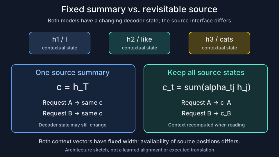
The baseline decoder state may still change. Attention adds a way to revisit stored source positions; both context vectors have fixed width. This is a schematic interface, not learned alignment.

4. From the current state to a set of reading weights

Denote the decoder state available before generating target token t by sₜ₋₁. It is a computed vector, not a handwritten instruction telling the model to “pay attention to cats.”

Following a Bahdanau-style order of computation, compare that state with every source representation using a learnable scoring function a_φ:

The symbol φ denotes the scorer’s parameters. Each score eₜⱼ is a real number used to determine how a candidate source participates in the current reading. It is not yet a probability, and it has no intrinsic semantic unit.

Choose Softmax to turn these scores into reading weights:

With at least one source position and finite scores, the weights are positive and sum to one. Use them to combine the source representations into a context vector for this step:

These are the three operations of the soft attention discussed here: compare the current state with available content, normalize the scores, and read the content through a weighted combination. Bahdanau’s paper describes this as soft alignment that changes across target-generation steps.⁴⁷

The sum runs over source positions, not the output vocabulary. These weights determine how to combine source information. The decoder must subsequently form a separate distribution over possible target tokens.

Attention weights are not next-token probabilities, and the context vector is not a probability distribution. The context is a vector with the same dimension as the source representations; its components may be negative and need not sum to one.

Softmax is not the only mathematically possible choice. A weighted sum using raw scores is also computable, but permits negative weights and an arbitrary overall scale. Nonnegative, normalized weights make this particular read a convex combination of source vectors. Change the normalization, and the reading operation changes too.

This also explains “soft.” We do not first select a single position and read only that position. Several positions participate continuously: small changes to their weights change the context vector continuously. Discretely selecting the highest-scoring position behaves differently. Away from a switching boundary, small changes do not alter the selection; at a boundary, it jumps. The same ordinary gradient cannot simply be passed through that selection rule. Hard selection is not untrainable, but it needs different treatment; reinforcement learning was used in visual attention, for example.⁶

There is one more difference from the everyday idea of “looking only at what matters”: this form of global soft attention usually still scores every source position. Its aggregation is selective; its computation is not automatically sparse or cheaper.

5. How did early attention compute a match?

The scoring function remains unspecified. We need a way for the decoder state and a source representation to jointly determine a scalar score.

Bahdanau attention uses a small feed-forward network for this purpose, now commonly called additive attention. We write an explicit bias below. To keep the matrix directions consistent, individual states in this article are column vectors.⁷

Let source representations have dimension d_h, decoder states dimension d_s, and the scorer’s intermediate layer width d_a. Its parameters are

The score is

The two matrices project inputs of potentially different widths into a common intermediate space. Their sum passes through an elementwise nonlinearity; the dot product with v produces one scalar. These parameters can be trained without first specifying a human-designed scale of semantic relevance.

The tanh is doing more than making the expression look like a neural network. What happens if we remove it and keep a purely linear sum?

The score becomes

For a fixed target step t, the decoder state contributes only a constant added to every source score. Article 01 established that Softmax is invariant to a shared additive shift. The weights therefore reduce to

In this particular construction without the nonlinearity, the current decoder state’s influence on the reading weights disappears completely. The reading rule no longer depends on the current request.

The nonlinearity allows the two inputs to influence scores jointly, rather than contributing only a shared offset that normalization removes. This does not make tanh the only option: multiplicative interactions can also make a match depend on the current state. The point is why this construction needs more than the addition of two linear scores.

The same scoring parameters are shared across target steps and source positions. Even when the trained parameters remain fixed, changing the current state can change the reading weights.

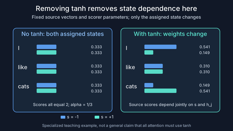
With exactly these fixed representations and parameters, removing tanh produces the same uniform source weights for both assigned states. With tanh, the weights change. Neither state is an executed decoder step.

6. The same content, read differently from a different state

Work through a small example.

Label the three source positions I, like, and cats. We specify their two-dimensional representations by hand. They are not pretrained embeddings or hidden states extracted from a real translation model:

For this example, shorten the decoder state to a scalar s and choose

Writing the two coordinates of each source representation as hⱼ,₁ and hⱼ,₂, the score expands to

Set state A to s = −1 and state B to s = 1, holding everything else fixed:

Using the unrounded weights, the two context vectors are approximately

The reading changes because its current state changes, not because we retrain the parameters or alter the source sentence.

Sweeping s across an interval shows how each source weight responds:

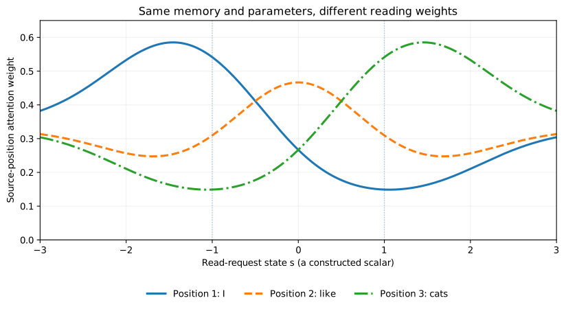
The horizontal axis is a constructed reading state, not training time or executed decoder steps. Each point evaluates the same attention function anew; these curves are not measured linguistic alignments.

The example establishes one thing: this differentiable computation can read the same content differently depending on its current state. It does not establish that s = −1 means “about to translate 我,” or that the model understands the sentence.

A large weight is not automatically the full causal importance of an input word either. A source representation can already contain information from other words, and the context vector will be processed further. A simple counterexample is a collection of identical source vectors: any weights summing to one produce the same context vector.

Attention weights describe how this computational node combines content. They do not, on their own, explain the entire prediction.

7. How does it learn where to look without alignment labels?

We chose the scoring parameters above. What would make them useful in a trained model?

The learning signal comes from the prediction objective used throughout this series.

Let y_t be target token t. In a model following the Bahdanau-style reading order, the decoder first obtains c_t, then uses it together with the previous state and the embedding of the preceding target token to update its state. Write the target-language embedding lookup as e_tgt. Schematically,

The token y₀ marks the start of the sequence. An output layer then uses the decoder state and other available information to form a distribution over the target vocabulary. The equation shows dependencies rather than reproducing every detail of the original output layers.⁴⁷

Let U be the target length, with the source still containing T tokens. Collect all trainable model parameters in θ, including the scorer parameters φ. Source and target lengths need not coincide. For one source–target pair, the loss can be written as

The actual target y_t is used to evaluate the loss; it is not supplied in advance as the answer to the same step’s attention computation. Training may supply previous ground-truth target tokens, a practice called teacher forcing. Supplying the past and revealing the token currently being predicted are different things.⁷

Prediction gradients propagate backward through the output computation to the context vector, reading weights, scorer, and encoder representations. In this setting, the scorer can be optimized jointly with the translation model without separately labeling which source position corresponds to each target word.⁴

We can derive part of that relationship directly. Treat the current context vector as a node in the computation graph, hold the source vectors fixed, and write the incoming gradient from subsequent computation as a column vector:

Differentiating Softmax and the weighted sum gives the sensitivity of this read to one source score:

Apply Article 03’s chain rule:

This explains part of what “learning where to look” means. If slightly increasing a source score would move the context vector in a direction that lowers the loss, the local gradient with respect to that score favors such a change. The gradient then continues into the shared scoring parameters.

This is the gradient through one reading operation with the source representations held fixed. Full training changes those representations too, and parameter updates reflect other decoder computations and examples. There is no promise that every update makes the alignment more consistent with human intuition.

The final prediction is supervised; how to read receives a learning signal through its effect on that prediction.

8. From early attention to another architecture

Attention no longer needs to mean one particular QKV equation.

In the model above, an RNN produces the source representations, the decoder supplies the current state, and attention combines source information accordingly. Recurrence has not disappeared; the reading mechanism was added to a recurrent model.

Luong and colleagues’ 2015 work retained LSTMs while exploring global and local reading, dot-product scoring, and scores involving a learned matrix. Its decoding order also differs from Bahdanau’s model. Merely replacing one scoring equation is not enough to reproduce the whole architecture.⁵

It helps to keep two questions separate: how the current state is formed, and how that state reads from the available content.

Likewise, the bidirectional source encoder here may read the entire source sentence because it is already available in offline translation. That does not give it access to future target tokens. Reading inside an autoregressive language model requires a separate decision about which positions are visible. There is no single mask to impose indiscriminately on every attention mechanism.

We can now ask the next questions. If every position needs to read, could all positions make their own requests? Must the representation used to score a match be the same representation that is ultimately retrieved? Must a recurrent network organize those requests first?

These questions lead toward self-attention, Q/K/V, and the way a Transformer updates its representations. Before introducing them, the idea developed here is already concrete:

Keep a collection of representations accessible, use the current state to determine a reading, and use that reading in the next prediction.

QKV is one way to organize this idea, not a necessary starting point for understanding attention.

Reproduce the numerical example and its gradient checks.