How Does Text Become a Vector?

English · 中文 · Français

First Principles of LLMs & RL · Article 04 · Previous article

Writing note: The questions and editorial direction are the author’s. ChatGPT assisted with drafting, mathematical checks, figures, editing, and translation.

From Tokenization to Learned Embeddings and Position

The first three articles explained how a model produces probabilities, how a loss evaluates its predictions, and how gradients change its parameters. But the inputs were mostly treated as numbers that somehow already existed. We could ask how those numbers should change without yet asking where they came from.

On the screen, I like cats is text. Matrix multiplication operates on numerical arrays. How do we get from one to the other, and how do we make those numbers useful to the model?

“Computers only understand numbers, so we need embeddings” is not enough. Token IDs are already numbers. An ID, however, tells the model which unit it has encountered, not how that unit should be represented. We have to separate three decisions: what units the text is divided into, how those units are identified, and how those identities receive learnable representations.

That distinction is a better starting point than a scatter plot of supposedly related words.

1. First decide what the model reads

Tokenization turns a piece of text into a sequence of units that the model will process. These units may be words, characters, subwords, or byte-based fragments. A token need not correspond to a linguistic word. BPE, WordPiece, and Unigram are representative ways to construct subword vocabularies, but they are different algorithms.¹

With a vocabulary consisting only of complete words, cat and cats could be separate entries. What happens when new names, inflections, and spellings appear? Collapsing them into the same unknown token loses distinctions. Character-level tokenization is more flexible in another sense, but can produce much longer sequences.

Subword methods offer a compromise. Consider a simplified, character-level version of Byte Pair Encoding (BPE): begin with individual characters within each word, count adjacent symbol pairs, merge the most frequent pair, and repeat. The result is an ordered set of merge rules. New text is processed with the learned rules; the tokenizer does not train a new set of merges for every input.²

Take a toy corpus containing four word forms: cat five times, cats three times, dog four times, and dogs twice. We forbid merges across word boundaries; ties are broken by the first pair encountered in our specified traversal. The first four merges are:

c + a  → ca       8 occurrences
ca + t → cat      8 occurrences
d + o  → do       6 occurrences
do + g → dog      6 occurrences

After those four merges:

cats → [cat, s]
dogs → [dog, s]

This is a fully specified teaching tokenizer, not the output of a real LLM tokenizer. The results happen to resemble stems and endings, but frequency, not grammatical morphology, drives BPE. The available base symbols, treatment of spaces, and possible use of bytes all affect a production tokenizer.¹

No word embedding has been produced yet. We have only decided which discrete units the model will see.

For the classical word-embedding examples below, switch explicitly to a different, word-level vocabulary, reusing our earlier toy words:

I → 0     like → 1     cats → 2     dogs → 3     pizza → 4

I like cats → [0, 1, 2]

These IDs belong to this word-level vocabulary, not the BPE vocabulary above. Whether our units are words or subwords, the next question is the same: how can their IDs participate in useful numerical computation?

2. An identity is not yet a representation

IDs 2 and 3 are adjacent integers. That says nothing about the meanings of cats and dogs. If the vocabulary IDs and their associated parameters are permuted consistently, the model can express the same computation.

One unambiguous representation is a one-hot vector. In our five-item vocabulary, cats is represented by the following row vector:

It identifies the category precisely. But every pair of distinct one-hot vectors is orthogonal, and every pair has Euclidean distance equal to the square root of two. The encoding has not specified which categories might share features.

Instead, introduce a learnable table. Let the vocabulary contain M entries, with d numerical features per entry:

For a token w, retrieve the row indexed by its ID:

An embedding here maps a discrete identity to a numerical feature vector the model can use. This particular mapping is a lookup into a table. Its entries are trainable real-valued parameters; the integer IDs themselves need no derivative. PyTorch’s Embedding implements this lookup operation.³

For illustration, suppose we choose this table by hand:

Looking up IDs [0, 1, 2] selects the first three rows, yielding a 3×2 matrix: three token positions, each with a two-dimensional representation. Repeating ID 2 retrieves the same parameter row.

These values may be negative and need not add up to one. An embedding is not a probability distribution, and it is not a set of output logits. It supplies features from which later computations may produce logits.

There is also a simple matrix identity behind the lookup:

Because the one-hot row has a single nonzero entry, multiplying by E selects one row. In practice, there is no need to allocate a full one-hot matrix.

This also shows that lookup is not the only way a neural network can process discrete symbols. A one-hot input followed by a trainable linear transformation can implement exactly the same mapping. The benefit is not a mysterious conversion that computers require. The representation lets many tokens share a finite set of numerical features; downstream parameters can operate on these features even when d is much smaller than the vocabulary size. This is one motivation behind distributed representations in neural language modeling.⁴

But we chose the numbers above by hand. The table is ready for computation, not automatically rich in linguistic structure. We can initialize embeddings and let a training objective change their values.

How an embedding is represented is a modeling choice. What its values become depends on the data and the objective used to learn them.

3. What evidence can give vectors useful structure?

A word’s neighboring words provide directly observable evidence.

Return to our five sentences:

I like cats
I like dogs
I like cats
I like pizza
I like cats

Define a context window containing the immediately adjacent word on each side, without crossing sentence boundaries. Let C_wc count how often context word c occurs next to center word w. For example, cats has like as a neighbor three times; dogs has it once.

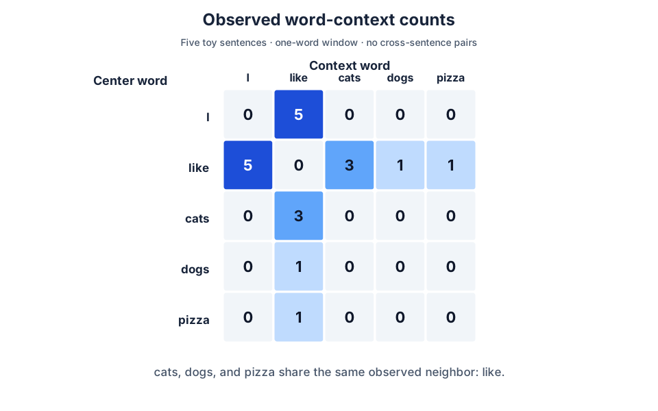
Each cell is an observed count under the declared window, not a learned similarity score.

A row of this matrix is already a vector representation. Its coordinates correspond to context words and its values to observed counts. As the vocabulary grows, however, these vectors are wide, sparse, and affected by common-word frequency.

Classical matrix-based approaches can weight, transform, and reduce such statistics. Latent Semantic Analysis (LSA), for example, applies low-rank factorization to term–document matrices. Word-context statistics can also be transformed using PPMI and reduced using SVD. Neural networks are not the only way to construct vectors.⁵

The tiny corpus also reveals a limitation. cats, dogs, and pizza only have like as a neighbor. Their normalized context-count rows therefore define identical context distributions.

That does not mean “cats, dogs, and pizza mean the same thing.” It means these data, under this context window, do not provide enough evidence to distinguish them. Learning from context is always limited by which observations and training tasks are actually available.

We can now use the same evidence differently: rather than treating the count matrix as the representation, train vectors to predict observed contexts.

4. Word2Vec: learn vectors by making predictions

Word2Vec’s two well-known architectures reverse the direction of prediction. In I like cats, if like is the center word, CBOW uses I and cats as context to predict like; Skip-gram uses like to predict each observed neighbor, I and cats. Basic CBOW aggregates context vectors and does not preserve their order.⁶

The training signal comes from the text itself: there is no need for someone to label every pair of words as semantically similar or dissimilar. Predicting window neighbors is not the same task as autoregressive next-token prediction; the window may include words on either side of its center.⁶

Begin with the full Softmax objective

Consider a full-softmax Skip-gram-style model. It uses two trainable tables. An input table E provides a vector e_w for the center word; an output table U provides a vector u_j for each candidate context word j. Both have M rows of dimension d, but their parameters are distinct.

A dot product produces a score, and Softmax normalizes the scores over possible context words:

Vocabulary IDs run from 0 to M−1. If the observed context ID is c, this pair incurs the loss

This is precisely the scoring-and-learning structure from the previous articles. The difference is that scores now come from word vectors. The loss learns the vectors themselves, rather than merely learning how to use fixed vectors. The two sets of representations and full-softmax Skip-gram formulation appear in the original work.⁷

Why is this more than another storage format? An independent score for every center/context pair requires M² numbers. Two M×d tables instead use 2Md parameters to generate all scores through dot products. When d is much smaller than M, pairwise scores cannot be chosen entirely independently; they must share lower-dimensional structure. This restriction can be useful, but does not guarantee that every geometric distance becomes a measure of semantic similarity.

Having two vectors for one word does not mean it has two incompatible meanings. The vectors play different roles in the predictive computation.

Actually update an embedding once

Take an observed training pair from the corpus: center word cats, context word like. In our declared input table, the initial vector for cats is (0,0). To isolate how that single row learns, fix the output table for this one step:

Initially, every dot product is zero, so the predictive distribution is uniform over five candidates. The observed-context loss is

Article 03 derived the cross-entropy gradient with respect to Softmax logits. Applying the chain rule through the dot products gives the gradient with respect to the input vector:

The indicator equals one only for the actual context c. Our five output vectors sum to zero, so the gradient in this example is (−1,0). At learning rate 0.5:

Recomputing scores and probabilities, the probability of like increases to about 0.313728; the loss falls to about 1.159228.

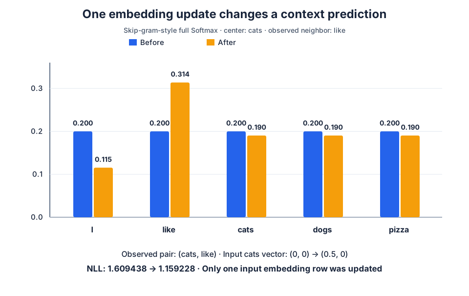
One specified gradient step, not pretrained embeddings or a measured training trajectory. No semantic cluster was invented.

We did not tell the model that the first coordinate should mean “liking.” The update simply makes an observed context more probable under this particular model. Full training would use many observed pairs and update both the input and output tables. U is fixed here solely to make one gradient calculation transparent.

Because the input table is shared, a later occurrence of cats retrieves the updated parameter row instead of creating a new vector.

Useful geometry emerges from constraints imposed by the learning task. Individual coordinates are not endowed with permanent semantic labels. If we applied the same orthogonal rotation to both the input and output vectors, all their dot products would remain unchanged; the predictive behavior would be identical.

Practical Word2Vec need not score the entire vocabulary

Full Softmax is convenient for understanding the mechanism, but requires scores for all candidate contexts. Word2Vec also used hierarchical softmax, and introduced negative sampling: training observed word pairs against pairs sampled from a noise distribution in a binary-classification-style objective. A sampled “negative” does not mean the pair can never occur in natural language.⁷

Negative sampling changes the objective. It is not simply full Softmax with a few denominator terms omitted. Our full-softmax example explains the common foundation, without pretending the objectives are identical.

5. GloVe and fastText: change the evidence or the unit of parameter sharing

Word2Vec demonstrates how prediction can shape vectors. But predicting individual word pairs is not the only use of context evidence, and storing one independent input row per complete word is not the only parameterization.

GloVe fits aggregated co-occurrence statistics

GloVe begins with accumulated, corpus-wide co-occurrence counts. Continue to write C_ij for the count for word i and context j, and e_i and u_j for two vector sets. Introduce scalar biases b_i and c_j and a nonnegative weighting function ω. Over positive-count pairs, its objective can be written as

This is weighted squared error: a vector dot product plus biases is trained to approximate the logarithm of the co-occurrence count, with a weighting function controlling the influence of different counts. It is neither a literal saved frequency table nor a per-neighbor cross-entropy objective.⁵

Skip-gram turns observations of co-occurrence into predictive training pairs; GloVe directly fits aggregated statistics. Both exploit related evidence, but through different objectives. Neither follows uniquely from the abstract idea of “meaning.”⁸

fastText shares parameters across character fragments

With a table keyed only by complete words, the input vectors for cat and cats can be entirely independent. Their similar spellings do not directly enter the parameterization.

The fastText word-vector method learns vectors for character n-grams and combines them into word representations. To keep the picture small, look only at trigrams and add the boundary markers < and >:

cat  → <ca, cat, at>
cats → <ca, cat, ats, ts>

These are overlapping features: both words contain <ca and cat, so they share the corresponding parameters. The original method also includes a whole-word feature and uses several n-gram lengths, omitted from this illustration.⁹

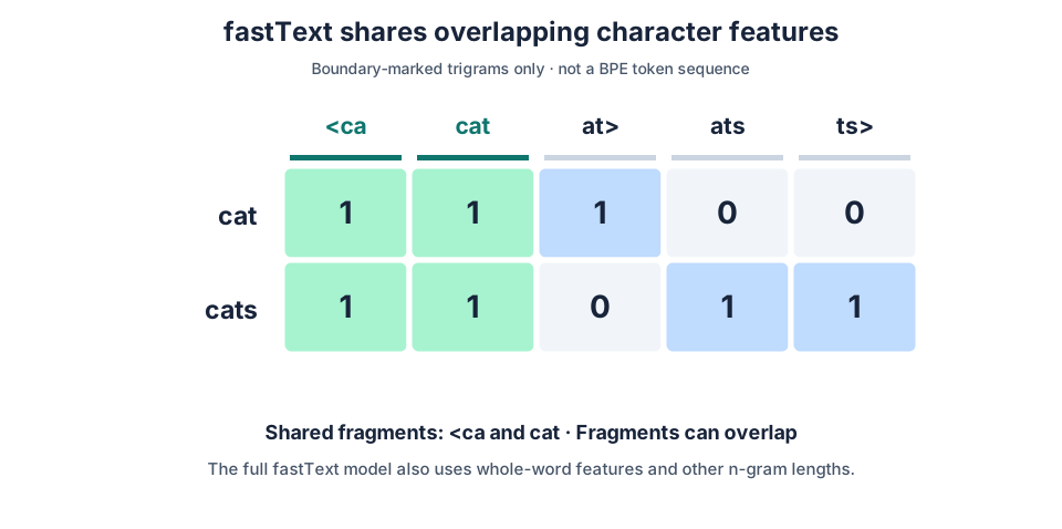
An entry of 1 means the fragment is present. This is not a token sequence, and it includes only length-three character fragments.

Let G(w) be the set of features used for word w, with a_g denoting the vector for feature g. The composition can be expressed as

Even if the full word has never appeared in training, its character fragments can supply a representation. This supports unseen word forms but does not guarantee that their meanings can be inferred reliably from spelling.⁹

fastText character n-grams and BPE subword tokens do different jobs. The former combine multiple, potentially overlapping fragments to represent a word; the latter determine a sequence of discrete input tokens. The shared term “subword” can obscure this distinction.

Word2Vec, GloVe, and fastText are different answers to the same broad problem: how to learn useful word representations from evidence, with different objectives and different granularity of parameter sharing.

6. What does “embedding” mean in an LLM?

Separate how a vector was learned from how it is retrieved during a computation.

For a conventional embedding lookup, holding the parameters fixed, the same ID retrieves the same row. This is the sense in which traditional word embeddings are called static: the lookup does not recompute the vector for the current sentence. Those parameters can, of course, change during training.

An LLM can also have a learned input token embedding table. Whether its vocabulary is based on words, subwords, or byte-related tokens, the lookup relationship is the same. Its vectors may be trained jointly with the language-model prediction objective; there is no requirement to train Word2Vec separately first.⁴¹⁰

The input table and the model’s later, context-dependent hidden representations are different objects. Compare:

I like
They like

If like corresponds to the same token ID, the lookup alone returns the same row. After a network has processed the two different prefixes, however, its hidden representation at like may differ because the context is now different.

An input embedding is a row of a parameter table. A contextual representation is computed for this particular input. The latter changing from context to context does not require changing the former during inference. We leave that contextual computation unopened until the next article.¹⁰

The output side of a language model must also map hidden representations to vocabulary scores. Some architectures tie the input table and output weights. For a hidden row vector h of the same width as the embedding, and omitting bias for simplicity, that can be written as

This returns a score for each candidate token, not one retrieved embedding row. Weight tying is a design choice, not a mathematical inverse of embedding lookup.¹¹

Sentence and document embeddings used in retrieval introduce another level. A variable-length text must be encoded and summarized into a fixed-size vector; specialized training objectives may be needed to make vector similarity useful for retrieval. Sentence-BERT is one example. There is no row in a token embedding table that can simply be looked up for an arbitrary whole sentence.¹²

Thus “embedding” may refer to a token’s input parameters, a context-dependent representation at a position, or a vector summarizing a sentence or document. The shared word does not mean these objects are interchangeable—or that any vector is automatically suitable for semantic search.

7. We have vectors. Where is word order?

One issue remains: position.

For now assume word-level tokenization again, and compare:

dog bites man
man bites dog

If we simply sum their three word vectors, both sentences yield the same result, because addition does not depend on order. The problem is not poor vectors: it is that our chosen aggregation has discarded the sequence.

Putting a token in a particular row of a matrix and making the computation use that row index are different things. We need to give the model a usable signal about where a token occurs rather than expect a word vector to represent all of its possible positions.

Learned absolute position embeddings

One approach assigns trainable vectors to absolute positions. Suppose we prepare up to L positions, each with d features:

Let x_i be the token ID at position i. In a model that adds position and token representations:

The same token at a different position can have a different initial representation. E is indexed by token ID; R by position. Addition preserves the feature width. It is a modeling choice, not a requirement imposed by probability theory. The original Transformer discussed both learned position embeddings and fixed sinusoidal encodings.¹⁰

A learned table provides position parameters, but merely having rows for rarely trained positions does not guarantee that the model will use them reliably.

Fixed sinusoidal position encodings

We can instead calculate positional vectors from functions, without learning a separate table. Let d be even, position i start at zero, and r range from zero to d/2−1:

Every coordinate pair has a shared frequency, while different pairs change at different rates. The original Transformer used this fixed encoding. The constant 10000 is a design scale, not something forced by the definition of position.¹⁰

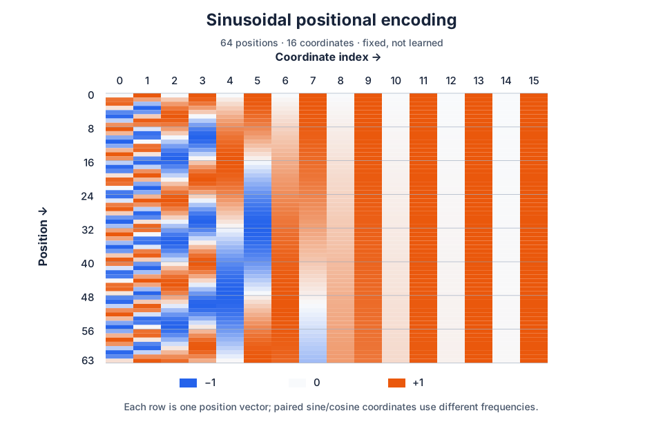
Rows are positions; columns are feature coordinates. The values come from the formula, not a training run.

Nearby positions consequently have structured numerical differences rather than unrelated identities. The angle-addition formulas for sine and cosine also make fixed positional offsets expressible through linear relations. Still, the ability to calculate an encoding at a farther position does not guarantee that the trained model works reliably on longer contexts. Having a mathematically defined input and generalizing to that input are different matters.

A subtle limitation is worth checking: if we add positional vectors, does every subsequent aggregation automatically preserve word order?

No. If we immediately sum across all positions,

For two equal-length sentences differing only by a permutation of the tokens, this expression is unchanged.

Position encoding supplies information that can be used. The downstream computation must actually use it before discarding the correspondence between tokens and positions. Word vectors plus position vectors alone do not explain a whole language model.

Positional information need not be added to token embeddings

The terms positional embedding and positional encoding overlap in practice. A more useful distinction is whether the representation is learned, whether it concerns absolute or relative position, and where it enters the computation.

Some methods inject relative position into the matching between sequence positions. RoPE uses position-dependent rotations in a later matching operation; ALiBi adds a bias related to positional distance to the matching scores, rather than adding another table to the input embedding.¹³¹⁴

Deriving these mechanisms properly requires the Attention computation in the next article. The boundary here is important: not every positional mechanism has the form “token embedding plus positional embedding.” Our example of an order-invariant sum does not prove that every architecture without explicit added position vectors is incapable of using order.

8. What is still missing after text becomes vectors?

We can now turn text into a numerical matrix with T rows and d columns: T is the number of tokens emitted by our tokenizer, d the representation width. Each row has a defined origin. The table’s parameters can be adjusted by a training loss, and the model can choose how to incorporate position.

Return once more to I like and They like. If like has the same token ID and occupies the same position, token lookup plus the same absolute positional addition still produces the same initial vector.

Those two operations have not allowed it to read I or They.

Embedding gives discrete symbols learnable numerical representations. It does not, by itself, make a position interact with its context. The next article asks how a position can retrieve information from other positions and integrate what it retrieves into its own representation.

The figures illustrate constructed examples, not pretrained embeddings or experimental results. Reproducible calculations.