First Principles of LLMs & RL · Article 03 · Previous article
Writing note: The questions and initial draft material are mine. ChatGPT assisted with structuring, editing, figures, and translation.
From local approximation to gradient descent and backpropagation
The previous article explained how cross-entropy measures a model’s prediction loss. But computing a loss does not change the model’s parameters.
A number can tell us how poor the current prediction is. It does not arrive with instructions about which parameter to increase, which to decrease, or by how much.
Between measuring an error and modifying the model, we need an account of how the error changes.
I want to follow that missing link. First, what does a small parameter change do to the loss? Then, which changes would be favorable? Finally, how do we calculate those sensitivities when the parameters are separated from the loss by a long chain of computations? Taylor expansion, gradient descent, and backpropagation answer these questions in sequence.
1. A loss value has no direction. A derivative does.
Set the network aside for a moment. Suppose there is only one real parameter, and the loss is
\[L(\theta)=(\theta-3)^2.\]At parameter values 1 and 5, the loss is 4 in both cases. Yet to approach the minimum, we should increase the former and decrease the latter. The loss value alone cannot distinguish these situations.
The derivative supplies the missing information:
\[L'(\theta)=2(\theta-3).\]At parameter value 1, it is −4. That does not mean the loss is negative. It means a sufficiently small increase in the parameter will decrease the loss at this point.
This interpretation follows almost directly from the definition of a derivative. Let δ be a small change to the parameter:
\[L'(\theta) = \lim_{\delta\to0} \frac{L(\theta+\delta)-L(\theta)}{\delta}.\]For sufficiently small δ, we can approximate the change in loss by
\[L(\theta+\delta) \approx L(\theta)+L'(\theta)\delta.\]For example, starting at 1 and increasing the parameter by 0.01, the first-order approximation predicts a loss of 3.96. Evaluating the original function gives 3.9601.
The approximation is not exact, but it captures the effect of this small change.
A derivative is not the size of the current error. It is the local sensitivity of the loss to a change in a parameter. Equal loss values may have entirely different sensitivities.
2. Taylor expansion: using local information to reconstruct nearby behavior
The approximation above is already a first-order Taylor approximation. It replaces the function near the current point with a line having the same value and slope there.
If a line matches height and slope, could a polynomial also match curvature?
Let f be a scalar-valued function, a the point around which we expand, and δ the displacement from a. Start with a quadratic polynomial:
\[p_2(\delta)=c_0+c_1\delta+c_2\delta^2.\]Require that its value and its first two derivatives at zero match those of f at a:
\[c_0=f(a),\qquad c_1=f'(a),\qquad 2c_2=f''(a).\]Then
\[f(a+\delta) \approx f(a)+f'(a)\delta+\frac{f''(a)}{2}\delta^2.\]The factor one half is not an arbitrary convention. Differentiating a quadratic term twice produces a factor of 2, which has to be canceled when we match the second derivative. Matching higher derivatives produces the corresponding factorials.
More generally, let n be the highest polynomial degree and denote the remainder by Rₙ:
\[f(a+\delta) = \sum_{k=0}^{n}\frac{f^{(k)}(a)}{k!}\delta^k +R_n(\delta).\]Here n is a nonnegative integer and the zeroth derivative is the function itself. This is an identity with a remainder. It becomes a useful approximation only when that remainder can be controlled.
For instance, suppose the (n+1)st derivative is continuous on the interval of interest, and its absolute value is at most M. Taylor’s theorem gives
\[|R_n(\delta)| \leq \frac{M}{(n+1)!}|\delta|^{n+1}.\]Under these assumptions, small displacements control the error. None of this says that the infinite Taylor series of every smooth function converges to that function.1
The point of Taylor expansion is to construct a simple approximation to nearby behavior from derivatives at one point.
Consider the exponential function expanded around zero:
\[e^x\approx1+x+\frac{x^2}{2}.\]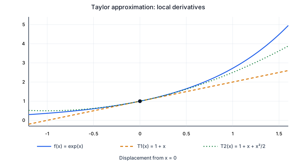
The approximations match increasingly many derivatives at the expansion point. They are not the same function everywhere. The horizontal axis is the displacement from zero.
At x = 0.2, the first-order approximation gives 1.2, the second gives 1.22, and the true value is about 1.2214. At x = 1, the same approximations give 2 and 2.5, while the true value is about 2.7183.
I deliberately chose a nonquadratic function for this graph. A quadratic’s second-order Taylor polynomial equals the original function everywhere, hiding the limitations of approximation.
Now return to learning. If a local approximation lets us predict the effect of a small parameter change, which change should we choose?
3. Why the negative gradient, and why does step size still matter?
A network has many parameters. Write them as an m-dimensional real vector in bold, and for now hold the training data, random choices, and the current computation fixed, so that the loss is a deterministic function of that vector.
The partial derivatives form the gradient:
\[g=\nabla L(\boldsymbol\theta) = \begin{bmatrix} \frac{\partial L}{\partial\theta_1}\\ \vdots\\ \frac{\partial L}{\partial\theta_m} \end{bmatrix}.\]At a differentiable point, the multivariable first-order approximation becomes
\[L(\boldsymbol\theta+\Delta\boldsymbol\theta) -L(\boldsymbol\theta) \approx g^\top\Delta\boldsymbol\theta.\]The right side is an inner product: each parameter change is multiplied by its local sensitivity, and the contributions are added. A gradient therefore evaluates an entire small update, not merely separate coordinates.
To talk about the steepest descent direction, we must decide how to compare the lengths of directions. Use Euclidean length, with u denoting a unit vector. By Cauchy–Schwarz,
\[g^\top u\geq-\|g\|_2, \qquad \|u\|_2=1.\]If the gradient is nonzero, equality holds when
\[u_*=-\frac{g}{\|g\|_2}.\]Among equally small changes measured by Euclidean length, the negative gradient has the greatest instantaneous rate of decrease. “Steepest” depends on how length is defined; it is not a coordinate-free absolute statement.2
The simplest gradient descent rule scales the negative gradient by a positive learning rate η:
\[\boldsymbol\theta_{t+1} = \boldsymbol\theta_t-\eta\nabla L(\boldsymbol\theta_t).\]Putting the proposed change back into the first-order approximation gives
\[L(\boldsymbol\theta-\eta g)-L(\boldsymbol\theta) \approx -\eta\|g\|_2^2.\]For nonzero g, the right side is negative. But it only tells us about sufficiently small steps: the approximation was built at the current point, not at every point we might reach.
The gradient indicates which way a small step should go. The learning rate determines how far the actual step goes.
Return to the parabola, starting at parameter value 1. The derivative is −4, so the next parameter is
\[\theta_{\mathrm{new}}=1+4\eta.\]| Learning rate η | New parameter | New loss | Compared with initial loss 4 |
|---|---|---|---|
| 0.10 | 1.4 | 2.56 | Lower |
| 0.75 | 4.0 | 1.00 | Overshoots the minimum, still lower |
| 1.00 | 5.0 | 4.00 | No improvement |
| 1.10 | 5.4 | 5.76 | Higher |
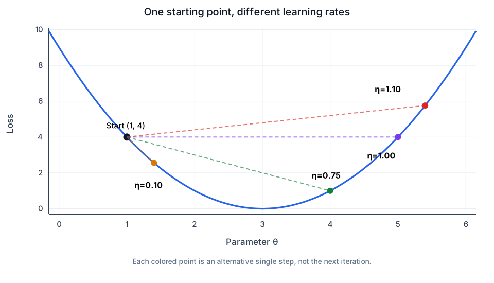
These arrows compare alternative single updates from the same starting point. They are not successive iterations in one training run, and the line connecting endpoints is not a continuous optimization trajectory.
For this particular quadratic, we can even derive exactly when the error shrinks:
\[\theta_{t+1}-3=(1-2\eta)(\theta_t-3).\]A fixed learning rate strictly between 0 and 1 makes the error shrink; η = 1 makes a nonoptimal point oscillate between two positions, and η > 1 makes the error magnitude grow. This range belongs to this function and must not be used as a universal learning-rate rule.
The difference between local and global optimization is just as important. At a differentiable point with nonzero gradient, some sufficiently small step along the negative gradient decreases the loss. That alone does not guarantee convergence, or even convergence to a local minimum. A zero gradient may also indicate a local maximum or saddle point.2
Convexity supplies additional global structure: for an unconstrained differentiable convex objective, a point with zero gradient is globally optimal. Whether a particular algorithm reaches such a point requires further conditions. In general, “gradient descent at least guarantees a local optimum” is not a valid claim.
So far, we have assumed the gradient is already available. But a parameter does not directly produce the loss. Many computations lie between them. How are all those derivatives obtained?
4. Backpropagation: tracing sensitivity through a computation
Suppose a parameter first passes through φ to produce u, and the final loss is obtained by applying f:
\[u=\phi(\theta),\qquad L=f(u).\]A small parameter change first changes u and then changes the loss:
\[\Delta u\approx \phi'(\theta)\Delta\theta, \qquad \Delta L\approx f'(u)\Delta u.\]Combining the steps and taking the limit gives the calculus chain rule:
\[\frac{dL}{d\theta} = \frac{dL}{du}\frac{du}{d\theta}.\]Sensitivities multiply along a computational path because the change produced at one stage is magnified, reduced, or reversed at the next.
This chain rule is not the probability chain rule of Article 01. One differentiates compositions of functions; the other factorizes joint probabilities. Both operate stepwise, but they are different statements.
If a parameter influences the loss through several paths, we must include all of them. The paths’ contributions add where they meet.
Backpropagation organizes these relations on a computational graph. In the forward pass, each node computes an intermediate value. Working backward from the loss, we propagate derivatives in the reverse order of dependencies. Derivatives already computed for a shared intermediate node are reused instead of being recomputed from scratch for each parameter.3
Backpropagation also does not mean perturbing one parameter at a time and rerunning the network to estimate slopes. That would be finite differences, which can check a small example. Here we differentiate the operations composing the graph and assemble their derivatives with the chain rule.
Backpropagation computes gradients; an optimizer uses those gradients to update parameters. A model does not move simply because its gradients have been computed.
We can now make that distinction concrete by returning to the very same distribution used in the first two articles.
5. One real update for cats, dogs, and pizza
Keep the context “I like”. Five observed continuations gave the empirical distribution
\[P=(0.6,0.2,0.2).\]The three candidates are cats, dogs, and pizza, in that order. The model produces logits z and a temperature-1 Softmax distribution:
\[Q_k=\frac{e^{z_k}}{\sum_{j=1}^{3}e^{z_j}}.\]Holding P fixed and using natural logarithms, define average negative log-likelihood as a function of logits:
\[\ell(z)=-\sum_{k=1}^{3}P_k\log Q_k.\]The average matters here. The total NLL of the five observations would have a loss and gradient five times as large; using the same learning rate would produce a different step.
Write Softmax inside the loss and use the fact that P sums to one:
\[\ell(z) = \log\left(\sum_{j=1}^{3}e^{z_j}\right) -\sum_{j=1}^{3}P_jz_j.\]Differentiating the first term with respect to the kth logit gives Qₖ; differentiating the second gives −Pₖ. Consequently,
\[\boxed{ \frac{\partial\ell}{\partial z_k}=Q_k-P_k }\]This is an exact result under the stated Softmax, fixed-target, and natural-log conventions, not a property of every imaginable loss.
Take the logits from the previous two articles:
\[z=(0,1,2).\]They give approximately
\[Q\approx(0.090031,0.244728,0.665241),\] \[\nabla_z\ell\approx(-0.509969,0.044728,0.465241).\]If the three logits could be adjusted independently, the negative-gradient step would raise cats and lower the other two scores. We now have a direction corresponding to the earlier intention of assigning observations more appropriate probabilities.
In a real network, however, we usually update shared parameters, not independent logits permanently stored for each context. For a worked example, construct a model with only one trainable scalar parameter:
\[z(\theta)=(2\theta,\theta+1,2).\]This is an intentionally limited teaching model, not a description of a full language-model architecture. At θ = 0, it reproduces the logits above.
One parameter affects both cats and dogs. Define the parameter-level objective
\[L(\theta)=\ell(z(\theta)).\]By the chain rule, the contributions along every output path must be added:
\[\frac{dL}{d\theta} = \sum_{k=1}^{3} \frac{\partial\ell}{\partial z_k} \frac{dz_k}{d\theta}.\]At θ = 0,
\[\begin{aligned} \frac{dL}{d\theta} &=2(-0.509969\ldots) +1(0.044728\ldots) +0(0.465241\ldots)\\ &\approx-0.975210. \end{aligned}\]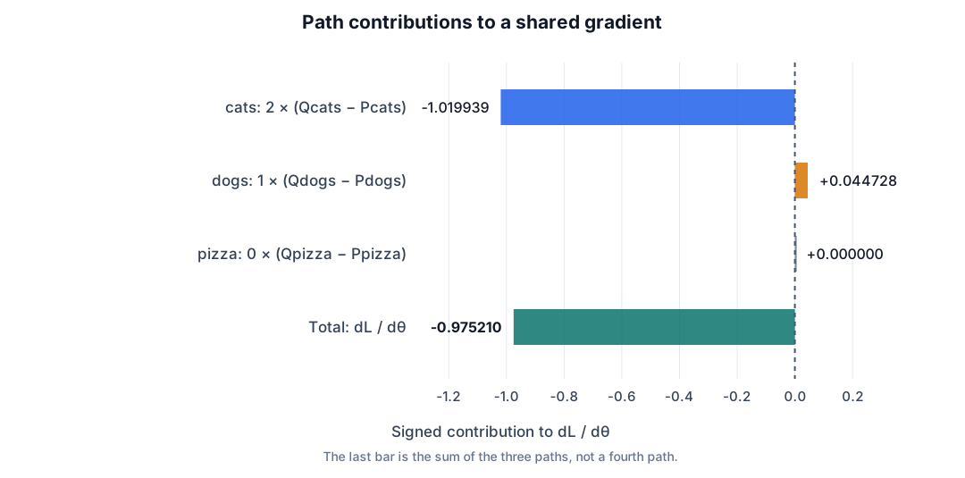
The three paths have different signed contributions. The bottom bar is their sum, not a fourth path. The pizza logit does not depend on θ, so that path’s local derivative is zero.
This is “multiply along a path, add at the point where paths meet” in numerical form. The cats path favors increasing the parameter; the dogs path favors decreasing it. Their total determines the parameter’s local update direction.
Now take one gradient descent step with learning rate 0.5:
\[\theta_{\mathrm{new}} =0-0.5(-0.975210\ldots) \approx0.487605.\]Recompute the logits, probabilities, and loss:
| Quantity | Before | After |
|---|---|---|
| θ | 0.000000 | 0.487605 |
| cats logit | 0.000000 | 0.975210 |
| dogs logit | 1.000000 | 1.487605 |
| pizza logit | 2.000000 | 2.000000 |
| cats probability | 0.090031 | 0.183291 |
| dogs probability | 0.244728 | 0.305965 |
| pizza probability | 0.665241 | 0.510743 |
| Mean NLL | 1.807606 | 1.389241 |
There is a detail worth noticing. Dogs already had a model probability above the empirical target 0.2; after the update, it increases even further.
That is not a contradiction. One shared parameter affects several logits at once; we do not have an independent dial for every probability. The objective minimizes the total P-weighted log-loss, not each class’s absolute probability error. This step reduces the former without improving every class’s match to P.
And although the pizza logit does not move, its probability does: the Softmax denominator depends on all logits.
A parameter update can reduce the overall loss without bringing every single predicted probability closer to its target in that step.
These are calculations from the specified equations, not claims about measured training performance.
6. Separating differentiation from an update in code
The same toy model fits into a short, typed PyTorch example:
import torch


def toy_logits(theta: torch.Tensor) -> torch.Tensor:
    """Map a scalar parameter to three shared logits."""
    return torch.stack((2.0 * theta, theta + 1.0, theta.new_tensor(2.0)))


def toy_loss(theta: torch.Tensor, target: torch.Tensor) -> torch.Tensor:
    """Return the average natural-log loss for a fixed target distribution."""
    log_probs = toy_logits(theta).log_softmax(dim=-1)
    return -(target * log_probs).sum()


target: torch.Tensor = torch.tensor([0.6, 0.2, 0.2], dtype=torch.float64)
theta: torch.Tensor = torch.tensor(0.0, dtype=torch.float64, requires_grad=True)
learning_rate: float = 0.5

loss_before = toy_loss(theta, target)
loss_before.backward()  # Compute gradients; theta is still zero.

if theta.grad is None:
    raise RuntimeError("The parameter gradient was not computed.")

with torch.no_grad():
    theta -= learning_rate * theta.grad  # Perform the parameter update.

theta.grad = None  # Do not accumulate this step's gradient into the next one.
loss_after = toy_loss(theta, target)

print(f"{loss_before.item():.6f} -> {loss_after.item():.6f}")
The checked output is
1.807606 -> 1.389241
backward() traverses the graph and accumulates derivatives in the leaf tensor’s .grad. It does not update θ. We perform the update inside no_grad(), and then run a fresh forward computation to obtain the new loss. Before the next backward pass, any gradients that should not accumulate must be cleared.4
Some parts of this story use approximations and some do not. Taylor approximates the effect of a finite displacement by a local polynomial. Backpropagation through this smooth computational graph instead computes derivatives at the current point by applying differentiation rules; it does not use a tangent line to guess each derivative. Floating-point computations naturally still incur numerical error.3
Only now do we have a training loop: a forward pass produces a loss, a backward pass produces sensitivities, an update rule changes parameters, and the next forward pass evaluates the new model.
We have not obtained a complete map to the optimal model. We have obtained a local procedure we can repeat.
The first two articles explained how to represent a distribution and how to define a loss. This one allowed that loss to influence shared parameters. Yet our toy model reduced the mapping from context to logits to something tiny.
The next article will open that box: how can a token retrieve useful information from earlier tokens, in a way that can be trained using the same loss?
-
OpenStax, Calculus Volume 2, Taylor and Maclaurin Series. Taylor polynomials, remainder bounds, and convergence of infinite series are distinct questions. ↩
-
Ian Goodfellow, Yoshua Bengio, and Aaron Courville, Deep Learning, Chapter 4: Numerical Computation, Section 4.3. All numerical results for the parabola are computed from the equation stated in the text. ↩ ↩2
-
Atilim Gunes Baydin, Barak A. Pearlmutter, Alexey Andreyevich Radul, and Jeffrey Mark Siskind, Automatic Differentiation in Machine Learning: a Survey, JMLR 18(153):1–43, 2018. See also PyTorch Autograd mechanics. Here we derive gradients through smooth operations; we do not discuss conventions at nondifferentiable points. ↩ ↩2
-
PyTorch documentation, torch.autograd.backward and Autograd mechanics. ↩