Why Does −log p Keep Appearing?

English · 中文 · Français

First Principles of LLMs & RL · Article 02 · Previous article

Writing note: The ideas and original draft material are mine. ChatGPT assisted with structuring, editing, and translation.

From Surprisal to Entropy, Cross-Entropy, and KL Divergence

In the previous article, we started with observations, passed through logits, Softmax, and the probability chain rule, and eventually arrived at a familiar term in language-model training:

\[-\log Q(y).\]

Here, Q is the probability distribution produced by the model, and y is the token that actually appeared. The less probability the model assigns to that observation, the greater the loss.

But the negative logarithm appears well beyond maximum likelihood. Information theory uses it to describe the information in one observed outcome. Taking its expectation gives entropy. If the distribution producing the data differs from the one used to predict them, we obtain cross-entropy. Subtracting the appropriate baseline leads to KL divergence.

Why do these quantities have such similar forms? One place to begin is a simple requirement: if two events unfold in succession, we want to be able to combine the information they provide.

1. Why is the information in an observation a negative logarithm?

Imagine two possible outcomes. One has probability 0.99; the other, 0.01. The first is hardly surprising when it happens. The second is a different matter.

If probability is going to determine information content, at the very least, a less probable outcome should carry more information, and a certain outcome should carry none.

There is a further requirement. Suppose event A happens, then we observe B knowing that A has occurred. The definition of conditional probability, which we used in the previous article, gives:

\[P(A\cap B)=P(A)P(B\mid A).\]

If we want the information in the combined event to equal the information from the first step plus the additional information from the second, we need a function that turns a product into a sum. The logarithm does exactly that:

\[-\log P(A\cap B) =-\log P(A)-\log P(B\mid A).\]

Notice that A and B need not be independent. Only under independence can the second term be replaced by the information in B without conditioning on A.

More generally, suppose a continuous information function satisfies:

\[I(pq)=I(p)+I(q),\]

and strictly decreases as the probability increases. Its form must then be a positive multiple of the negative logarithm. Choosing natural logarithms and setting that multiplier to one gives surprisal (self-information):

\[I_P(x)=-\log P(x),\qquad P(x)>0.\]

The subscript P matters: the same outcome may have different surprisal under different probability distributions. With logarithms to base 2, information is measured in bits; with natural logarithms, in nats (natural units of information). These are different scales for the same quantity.¹

For example, an event whose probability is exactly one over e carries:

\[-\ln(e^{-1})=1\ \text{nat}.\]

Changing the logarithm’s base gives the conversion:

\[1\ \text{nat}=\frac{1}{\ln2}\ \text{bits}\approx1.4427\ \text{bits}.\] \[1\ \text{bit}=\ln2\ \text{nats}\approx0.6931\ \text{nats}.\]

A fair coin produces either side with probability one-half. Observing a particular side therefore provides 1 bit, or approximately 0.6931 nats. The unit changes the number, not the coin’s uncertainty or the ordering of outcomes by surprise.

An outcome to which a model assigns exactly zero probability has infinite surprisal under the limiting convention.

None of this says that nature has decreed a logarithmic measure of information. The logarithm follows from the properties we ask information to have, particularly the additivity of information when probabilities multiply.

2. Why is entropy expected surprise rather than total surprise?

Entropy measures how much uncertainty remains about which outcome will occur next, even when we know the probabilities of all the possibilities. Numerically, it is the average self-information gained when the outcome is revealed.²

The qualification “even when we know the probabilities” matters. Knowing that a coin is fair does not tell us which side will come up next. Uncertainty about the outcome is different from uncertainty about the coin’s probability—or from a model’s lack of knowledge.

If one outcome is almost certain, the revelation usually tells us little. If several outcomes are plausible, the revelation carries more information on average. That intuition tells us what the expectation in the formula is for.

Return to the tiny corpus from the previous article. We observed five tokens after I like: three instances of cats, one dogs, and one pizza. Their empirical distribution is:

\[P=(0.6,\ 0.2,\ 0.2).\]

Here P is an empirical distribution used for illustration, not the unknown, true language-generating distribution. We omit the common conditioning context for now.

If the next observation is cats, its surprisal under P is:

\[I_P(\mathrm{cats})=-\log 0.6\approx0.511.\]

If we see dogs instead, it is:

\[I_P(\mathrm{dogs})=-\log 0.2\approx1.609.\]

The same distribution can produce outcomes with quite different surprisal. The information in a single observation depends on which outcome actually occurs; before observing it, we do not know what that value will be.

To describe the uncertainty of the distribution as a whole, ask how much surprisal we would get on average when drawing repeatedly according to P. That calls for an expectation:

\[\begin{aligned} H(P)&=\mathbb E_{X\sim P}[-\log P(X)]\\ &=-\sum_x P(x)\log P(x). \end{aligned}\]

For our three outcomes:

\[H(P)=-0.6\log0.6-2(0.2\log0.2) \approx0.950\ \text{nats}.\]

If an outcome has zero probability, its contribution to the entropy sum is defined by the usual limiting convention. This value is neither the 0.511 nats obtained from cats nor the 1.609 nats obtained from dogs. It is their probability-weighted average over all possible outcomes.

We can see the pattern more clearly by letting the probabilities of two outcomes vary:

\[P_p=(p,1-p),\qquad 0\leq p\leq1.\]

The corresponding entropy is:

\[H(P_p)=-p\ln p-(1-p)\ln(1-p).\]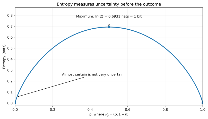

The horizontal axis changes the distribution parameter p, not the result of a particular trial. The vertical axis is the entropy of that distribution. At the endpoints, we use the limiting convention for zero-probability terms. The maximum is ln 2 ≈ 0.6931 nats, or 1 bit.

For a coin with probabilities 0.99 and 0.01, observing the rare side yields about 4.605 nats of surprisal, yet the entropy of the distribution is only about 0.056 nats. The rare event really is surprising, but it rarely occurs. An individual rare result can carry a great deal of information while the distribution’s average uncertainty remains low.

Why not just add up the surprisal of all possible outcomes? That would give equally rare and common outcomes the same weight; it would not answer how much information a typical draw provides. Accumulated information over n successive observations is a different quantity: for dependent outcomes, we add the conditional surprisal at each step given the previous outcomes, not blindly add the marginal surprises. For independent and identically distributed draws, the sample average converges to entropy under the usual conditions.

This also clarifies an easy confusion: expected surprise is not the same object as the surprise in each realized outcome. Their numerical values can coincide—under a uniform distribution, every possible outcome has surprisal equal to the entropy. But entropy characterizes the distribution, while surprisal characterizes a particular result. An empirical entropy computed from finite data need not equal the entropy of the unknown generating distribution.

What about entropy in physics? For a discrete distribution over a system’s microstates, Gibbs entropy has the same expectation-of-negative-logarithm structure:

\[S=-k_B\sum_i p_i\log p_i.\]

Here the probabilities refer to physical microstates and the Boltzmann constant has units of joules per kelvin. For that same microstate distribution, its relation to information entropy with natural logarithms is:³

\[\frac{S}{k_B}=-\sum_i p_i\ln p_i.\]

A two-microstate model can therefore reuse the shape of the binary-entropy curve above for S divided by the Boltzmann constant. The physical entropy S has units of J/K, however; this does not turn an arbitrary distribution over text tokens into the thermodynamic entropy of a physical system.⁴

If all Ω accessible microstates have equal probability, the formula reduces to Boltzmann’s familiar form:

\[S=k_B\log\Omega.\]

Physical entropy also depends on how microstates, energetic constraints, and thermodynamic quantities are defined. Simply calling entropy “disorder” does not explain why the expectation appears in its mathematical definition.

3. What if the data come from P but predictions use Q?

Entropy evaluates outcomes drawn from P using P’s own probabilities. In language-model training, however, the true distribution is unknown. We instead have a model distribution Q.

Keep the same three outcomes. Suppose the model produces logits:

\[z=(0,1,2).\]

Softmax turns them into:

\[Q\approx(0.0900,\ 0.2447,\ 0.6652).\]

Outcome	Empirical P	Model Q	Model loss if observed
cats	0.6000	0.0900	2.408
dogs	0.2000	0.2447	1.408
pizza	0.2000	0.6652	0.408

These are valid probabilities. But the model assigns the least probability to cats, the most frequent observation, and the most to pizza.

If outcomes still follow P but we use Q to predict them, how much negative log-loss should we expect on average?

\[\boxed{\begin{aligned} H(P,Q)&=\mathbb E_{X\sim P}[-\log Q(X)]\\ &=-\sum_x P(x)\log Q(x) \end{aligned}}\]

This is cross-entropy. The two distributions have different roles inside the expectation: P determines how frequently an outcome is encountered, while Q determines the loss assigned to that outcome.

For our example:

\[\begin{aligned} H(P,Q)&=-0.6\log0.0900-0.2\log0.2447\\ &\quad-0.2\log0.6652\\ &\approx1.808\ \text{nats}. \end{aligned}\]

The probabilities printed above have been rounded; the more precise result is approximately 1.8076 nats. We can display the expected loss as three separate, weighted contributions:

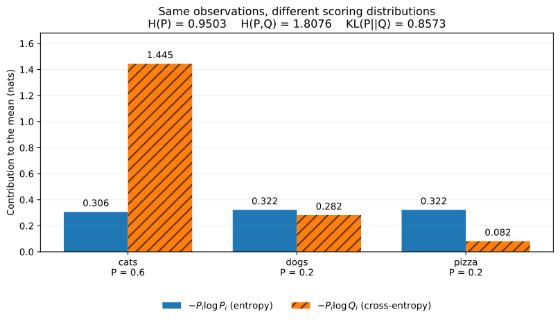
Each bar is one outcome’s contribution to the mean, not its raw surprisal. Summing the entropy bars gives about 0.9503 nats; summing the cross-entropy bars gives about 1.8076 nats. Both means use P as their weighting distribution. Only the probability inside the logarithm changes.

The total negative log-likelihood for our five observations is therefore approximately:

\[5H(P,Q)\approx9.038.\]

That is exactly the same calculation we performed at the end of the previous article. Because P was constructed from those five observed outcomes, empirical cross-entropy is average NLL.

Does cross-entropy still equal NLL with more than two classes? Yes, for a single one-hot label. If the observed class is y:

\[-\sum_{k=1}^{K}\mathbf 1[k=y]\log Q(k) =-\log Q(y).\]

With a full soft target distribution, cross-entropy is an expected NLL over that target, rather than the single term for one class.

The word cross can be understood as the fact that one distribution generates outcomes and another evaluates them. They may differ, but they may also happen to be the same. Cross-entropy is not another name for conditional entropy. Conditional entropy concerns two random variables and their joint distribution—for example, the remaining uncertainty about a token once its context is known. In H(P,Q), the arguments are distributions; in conditional entropy, the objects are random variables.

4. KL divergence: the additional cost of predicting with the wrong distribution

We now have two expected losses for outcomes drawn from the same distribution P. Scoring them using P gives entropy; using Q gives cross-entropy. Their difference is:

\[\begin{aligned} H(P,Q)-H(P) &=-\sum_xP(x)\log Q(x) +\sum_xP(x)\log P(x)\\ &=\sum_xP(x)\log\frac{P(x)}{Q(x)}. \end{aligned}\]

The right-hand side is KL divergence:

\[\boxed{ D_{\mathrm{KL}}(P\|Q) =\mathbb E_{X\sim P}\left[\log\frac{P(X)}{Q(X)}\right] }\]

Therefore:

\[\boxed{H(P,Q)=H(P)+D_{\mathrm{KL}}(P\|Q).}\]

For exactly the same P and Q:

\[\begin{aligned} H(P)&\approx0.9503,\\ H(P,Q)&\approx1.8076,\\ D_{\mathrm{KL}}(P\|Q)&\approx0.8573. \end{aligned}\]

KL is the additional expected log-loss incurred when we use Q instead of P to predict data generated by P. It does not follow from a universal decree that “model error must be measured by KL”. Once we adopt log-loss, KL appears as the gap above the best achievable average log-loss. Other loss functions give rise to other measures of mismatch.

A particular outcome may contribute less to cross-entropy than to entropy: our model, for instance, overestimates pizza, so predicting that outcome is relatively cheap. KL non-negativity concerns the total difference, averaged using P, not the contribution of each outcome separately.

We can keep P fixed and vary Q along a simple one-dimensional family. Let the model’s probability for cats be q, and divide the remaining probability equally between dogs and pizza:

\[\begin{aligned} P&=(0.6,0.2,0.2),\\ Q_q&=\left(q,\frac{1-q}{2},\frac{1-q}{2}\right),\quad 0<q<1. \end{aligned}\]

This family is chosen for the visualization; it is not the fixed Softmax distribution from logits (0, 1, 2).

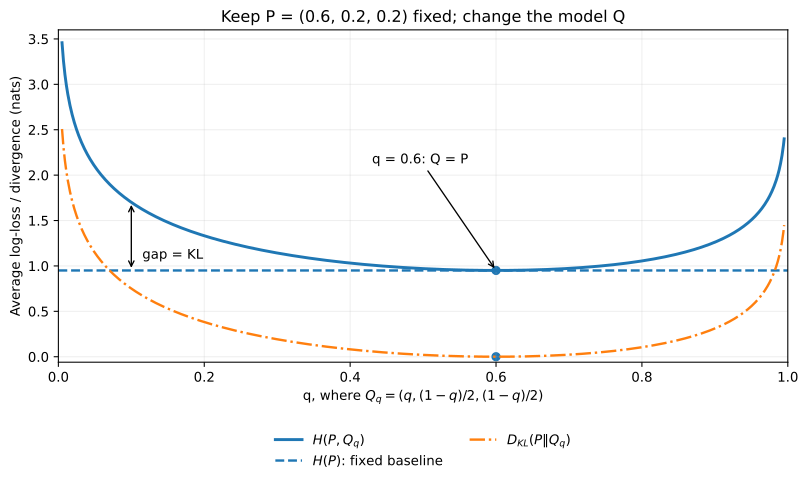
When q = 0.6, Q equals P, cross-entropy reaches H(P), and KL becomes zero. Since P stays fixed, H(P) is a horizontal baseline. Here the KL gap is a vertical difference between curve values, not an area between curves.

Why can the gap never be negative? Assume a finite outcome space and strictly positive P and Q. The elementary inequality for positive u is:

\[-\log u\geq1-u,\]

It gives:

\[\begin{aligned} D_{\mathrm{KL}}(P\|Q) &=\sum_xP(x)\left[-\log\frac{Q(x)}{P(x)}\right]\\ &\geq\sum_x(P(x)-Q(x))=0. \end{aligned}\]

Equality holds only when P equals Q. In other words, when data really follow P, using P itself to predict them cannot have a worse long-run average log-loss than using a different distribution.

But KL has a feature ordinary distances lack: direction matters.

\[D_{\mathrm{KL}}(P\|Q)\ne D_{\mathrm{KL}}(Q\|P)\quad\text{(in general)}.\]

Reversing the arguments for our same two distributions gives:

\[D_{\mathrm{KL}}(Q\|P)\approx0.6781,\]

as opposed to approximately 0.8573 in the forward direction. The difference is not a numerical trick: what matters is which distribution supplies the averaging weights. Forward KL averages over outcomes drawn from P; reverse KL averages over outcomes drawn from Q. Strictly speaking, reversing direction also inverts the ratio inside the logarithm; it is not just changing weights while keeping the integrand fixed.

An extreme case makes the directionality plain. If P assigns positive probability to an outcome but Q assigns exactly zero, forward KL is infinite; reverse KL need not be. Softmax with finite logits gives no exact zeros, but it can produce extremely small probabilities and correspondingly large penalties.

Further reading: what do mode-covering and mode-seeking mean?

A mode is a peak in a probability mass function or density. Imagine that the target distribution P has two well-separated peaks while the approximate distribution Q is restricted to a single Gaussian. Such a Q cannot reproduce both peaks, so an approximation must compromise.

Mode-covering describes a broad fit that tries to assign appreciable probability to several regions where P has significant mass. In this restricted example, minimizing forward KL often favors that compromise: P produces observations near both peaks, and missing one can carry a large log-loss.

Mode-seeking describes a fit that concentrates on one peak, even at the expense of missing another. Reverse KL averages under Q. Spreading Q widely across both peaks could put much of its mass in the valley where P is tiny; concentrating near one peak can avoid that penalty.⁵

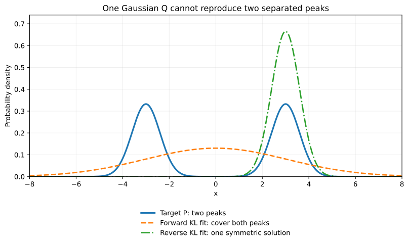
This is a separate example using continuous densities, not categorical next-token probabilities. The target is a 50/50 mixture of Gaussians centered at −3 and 3, each with standard deviation 0.6. The forward-KL optimum within the single-Gaussian family is obtained by matching moments. The reverse-KL curve is a solution found by multistart numerical optimization and independently checked by numerical integration—not a proof of global optimality. A symmetric counterpart exists at the other peak.

“Forward KL always covers every mode, while reverse KL always seeks one mode” is not a theorem. The behavior depends on P, the permitted family of Q, and the optimization result. If the approximation family contains P and we find that solution, both divergences can be zero. Mode is not synonymous with peak height; the preferred approximation depends on the probability distribution as a whole.

5. Back to language models—and a glimpse of RL

We can now put these relations back into a language model. Let C be the context, Y the observed next token, P_data the unknown data-generating distribution, and Qθ the model’s conditional prediction. Unlike the empirical distribution built from five observations, P_data denotes the underlying distribution. The population expected next-token NLL is:

\[\mathcal L(\theta) =\mathbb E_{(C,Y)\sim P_{\mathrm{data}}}\bigl[-\log Q_\theta(Y\mid C)\bigr].\]

Under suitable support assumptions, it decomposes as:

\[\begin{aligned} \mathcal L(\theta) &=H_{P_{\mathrm{data}}}(Y\mid C)\\ &\quad+\mathbb E_{C\sim P_{\mathrm{data}}} \left[D_{\mathrm{KL}}\bigl(P_{\mathrm{data}}(\cdot\mid C)\|Q_\theta(\cdot\mid C)\bigr)\right]. \end{aligned}\]

The first term is the conditional uncertainty inherent in the data distribution, and it does not depend on the model’s parameters. The second measures mismatch between the model’s conditionals and those of the data. Thus at the population-expectation level, minimizing cross-entropy is equivalent to minimizing forward KL with the data distribution in the first argument. In training we only approximate that expectation using finite samples; the true distribution is not handed to the model.

The same thread reaches maximum-entropy reinforcement learning, although I do not want to unpack a full RL algorithm here. Standard RL seeks policies with high expected reward. Entropy-regularized RL adds a weighted preference for retaining uncertainty in the policy distribution. Consider a simplified single-state problem with a finite action set and a known value score v(a) for each action. The policy π is a probability distribution over these actions: its probabilities are nonnegative and sum to one. We optimize:

\[\max_{\pi}\left\{ \sum_a\pi(a)v(a)+\alpha H(\pi) \right\},\qquad\alpha>0,\]

Introduce a Lagrange multiplier for normalization and differentiate with respect to each action probability:

\[v(a)-\alpha(\log\pi(a)+1)+\lambda=0.\]

Solving for their relative weights and normalizing yields:

\[\pi^*(a)=\frac{e^{v(a)/\alpha}}{\sum_b e^{v(b)/\alpha}}.\]

We have arrived at Softmax again. Reward still matters; encouraging entropy does not mean that the policy must keep choosing poor actions at random. It means trading off expected value against the possibility of several actions. Full dynamic RL also involves state distributions, future returns, and the temperature coefficient, which I will leave for a later article.

We started with the loss for one observation and ended with several different kinds of quantity: the surprisal of one outcome; the average surprisal of a distribution; the average log-loss of predictions based on another distribution; and the gap between those two averages. They share the negative logarithm but answer different questions.

The next time I see a negative logarithm, the first thing I want to ask is no longer just what the formula is called. It is: whose probability is inside the logarithm, and whose distribution determines the expectation?

The figures are teaching examples, not experimental results. Plotting source.