Where Do Probabilities Come From?
First Principles of LLMs & RL · Article 01 · Why this series?
Writing note: The ideas and original draft material are mine. ChatGPT assisted with structuring, editing, and translation.
From observations to Softmax and maximum likelihood
I understood how to expand the probability chain rule. What stopped me was a question before the algebra: where did the probability come from in the first place?
A training dataset contains things that happened: a sentence, a label, the next token after a particular prefix. A language model assigns probabilities to things that might happen. The dataset does not hand it a probability for every possible continuation.
There are two questions here. How do we construct a probability distribution from a network’s outputs? And how do observations tell us which distribution to prefer?
Softmax answers part of the first question. Maximum likelihood supplies a learning principle for the second. The probability chain rule connects their token-level and sequence-level views.
Observations, counts, and shared parameters
Consider five sentences. For this toy example, treat each word as one token:
I like cats
I like dogs
I like cats
I like pizza
I like cats
After I like, cats occurs three times; dogs and pizza occur once each. In that order, the empirical conditional distribution is
The hat marks an estimate constructed from the sample. The observations are the five sentences. The empirical distribution is a description we construct from them. It is not a complete account of how language is generated.
Counting continuations is closest to a count-based language model, not to Word2Vec. For example, let C(u,v) count how often token v follows token u, and let C(u) count occurrences of u with a following token. An unsmoothed bigram estimate is
\[\widehat P(v\mid u)=\frac{C(u,v)}{C(u)},\qquad C(u)>0.\]Longer contexts make direct counting sparse. A prefix may occur once, or not at all. Count-based models can address sparsity through smoothing and shorter contexts; neural language models instead learn distributed representations and probability functions that share information across examples.1
Word2Vec also learns vector parameters from word-context observations. Its embeddings are called static because a word’s lookup vector does not change with its surrounding sentence at use time, not because the vectors are a table of occurrence counts. They do change during training. Skip-gram learns input and output word representations; negative sampling is one of its training alternatives.2
For our language model, let c denote a context, y a candidate next token, and θ all model parameters. We want a function
\[P_\theta(y\mid c).\]Parameter sharing means that different contexts use the same parameter set, not that they receive the same output. An update from one example changes parameters also used for other examples. This creates an opportunity to generalize; it does not guarantee that generalization will be good.
Sharing and initialization are separate choices. In the from-scratch setting considered here, weight matrices start from a chosen random initialization; some other parameters can start at fixed values such as zero or one. Sharing is already part of the architecture before any training happens. Fine-tuning, by contrast, starts from previously learned parameters.
What exactly is a logit?
Calling a logit a “score” leaves an important question unanswered: a score of what?
Suppose a context has been mapped to a hidden vector h of dimension d. For candidate token i, an output layer can compute
\[z_i=w_i^\top h+b_i.\]Here wᵢ is a learned d-dimensional vector and bᵢ is a scalar bias. With K possible tokens, the outputs form
\[z=(z_1,\ldots,z_K)\in\mathbb R^K.\]These are the logits. At this point they are just unconstrained real numbers. They do not have a predefined unit of truth, confidence, or frequency. Their probabilistic interpretation comes from the way we choose to use them.
One useful choice is to interpret each logit as a log-weight. Exponentiating gives a positive weight:
\[a_i=e^{z_i}.\]Normalize those weights to obtain a categorical distribution:
\[p_i=\frac{e^{z_i}}{\sum_{j=1}^{K}e^{z_j}}.\]That is Softmax. For a finite vector of finite real logits, exact arithmetic gives strictly positive probabilities whose sum is one. A probability distribution in general may contain zeros; finite-logit Softmax represents its strictly positive interior.
A small example makes the transformation concrete. The entries below are rounded, but calculated from the same vector:
| Candidate | Logit | Positive weight after exp | Probability after normalization |
|---|---|---|---|
| A | 0 | 1.0000 | 0.0900 |
| B | 1 | 2.7183 | 0.2447 |
| C | 2 | 7.3891 | 0.6652 |
Think of allocating a fixed budget in proportion to positive weights. The weights need not sum to one; their shares do. Logits record those weights on a logarithmic scale. This is an analogy for the parameterization, not a claim that the network contains literal votes or evidence counters.
For a precise relationship, define the normalization constant
\[Z(z)=\sum_{j=1}^{K}e^{z_j}.\]Using natural logarithms throughout this article,
\[\log p_i=z_i-\log Z(z).\]A logit is a log-probability plus an offset shared by all candidates in the same distribution. That offset depends on the full logit vector. A logit by itself is therefore not a probability or a log-probability.
Softmax does not discover hidden probabilities inside arbitrary numbers. We choose it as a map from unrestricted scores to a distribution, then train the scores through that map. Even an untrained network can produce a valid distribution. Equal logits, for example, give
\[\operatorname{softmax}(0,0,0)=\left(\frac13,\frac13,\frac13\right).\]Random initialization need not produce exactly equal logits. The point is that a valid distribution can exist before the model has learned useful predictions. Normalization guarantees neither accuracy nor calibration. A next-token probability is also not automatically a probability that a statement is true.
Why exponentials, and why this base?
An obvious alternative is to divide scores by their sum. With arbitrary real scores, this can fail immediately:
\[\frac{(-2,1,3)}{-2+1+3}=\left(-1,\frac12,\frac32\right).\]The entries sum to one, but they are not probabilities. The denominator could also be zero.
Many positive functions avoid that problem. So positivity alone does not select the exponential. The more interesting property is how Softmax handles a shared offset. If a is any real constant and 𝟙 is the all-ones vector, then
\[\operatorname{softmax}(z+a\mathbf1)=\operatorname{softmax}(z).\]This follows because every exponential gains the same factor:
\[e^{z_i+a}=e^a e^{z_i}.\]That factor cancels during normalization. Scores (1, 2, 3) and (101, 102, 103) therefore define the same distribution. Choosing to ignore a common score baseline is a modeling preference; Softmax satisfying that preference is an algebraic fact.
There is a conditional characterization behind this. Suppose we apply the same continuous positive function g to each score and then normalize:
\[p_i=\frac{g(z_i)}{\sum_{j=1}^{K}g(z_j)}.\]Requiring invariance under every shared shift, and considering two scores u and 0, gives
\[\frac{g(u+a)}{g(a)}=\frac{g(u)}{g(0)}.\]Define h as the logarithm of g relative to its value at zero:
\[h(u)=\log\frac{g(u)}{g(0)}.\]The preceding relationship becomes
\[h(u+a)=h(u)+h(a).\]A continuous additive function is linear: additivity determines its rational arguments, and continuity extends the result to real arguments. Consequently,
\[g(u)=C e^{\alpha u},\qquad C>0.\]Requiring higher scores to receive higher weights additionally gives α > 0. The constant C cancels during normalization.
The exponential is singled out within this particular construction and its assumptions. Softmax is not the only possible map into a probability distribution.
The base is a separate issue. For any b > 1,
\[b^u=e^{(\log b)u}.\]Changing the base rescales the logits; it does not leave the probabilities of a fixed score vector unchanged. Natural exponentials and natural logarithms are convenient partners in calculus, but the important structure here is exponential weighting.
Differences are probability ratios
The most informative Softmax identity comes from comparing two candidates. Their normalization constant cancels:
\[\frac{p_i}{p_j}=e^{z_i-z_j}.\]Equivalently,
\[\boxed{z_i-z_j=\log\frac{p_i}{p_j}}\]A one-unit logit advantage means an e-fold probability ratio, not one extra percentage point of probability. Other candidates affect each individual probability, but not this pairwise ratio when the two logits are held fixed.
For two candidates, define
\[\Delta=z_1-z_2.\]Then
\[p_1=\frac{e^\Delta}{e^\Delta+1}.\] \[p_2=1-p_1.\]The graph below plots these two probabilities against the difference. Equal logits give equal probabilities. A difference of 1 gives approximately 0.7311 and 0.2689.
Move the slider to compare the probabilities. Open the interactive graph · Marimo source.
In the binary case only, the second probability is the complement of the first, so
\[z_1-z_2=\log\frac{p_1}{1-p_1}.\]This is the usual log-odds. With more classes, pairwise log-probability ratio is the less ambiguous description.
Temperature changes the scale of this relationship. For a positive temperature τ,
\[p_i^{(\tau)}=\frac{e^{z_i/\tau}}{\sum_{j=1}^{K}e^{z_j/\tau}}.\]Therefore,
\[\log\frac{p_i^{(\tau)}}{p_j^{(\tau)}}=\frac{z_i-z_j}{\tau}.\]A smaller positive temperature amplifies nonzero differences; a larger one compresses them. Temperature controls how strongly a score difference becomes a probability ratio. It does not change which score is largest.
Conditional probability is where the chain rule comes from
We now have a distribution for the next token. To assign a probability to a sequence, return to conditional probability itself.
Let A and B be events, with P(A) positive. The definition is
\[P(B\mid A)=\frac{P(A\cap B)}{P(A)}.\]We restrict attention to the probability mass inside A and ask what fraction also belongs to B. Rearranging gives
\[P(A\cap B)=P(A)P(B\mid A).\]For example, if A has probability 0.4 and B occurs within A with conditional probability 0.25, their intersection has probability 0.1. No independence assumption was needed.
For a fixed-length sequence, let T be the length. Write its observed token values as x₁, …, x_T, and define the prefix notation
\[x_{<t}=(x_1,\ldots,x_{t-1}).\]Repeatedly apply the same conditional-probability identity to prefixes, assuming the conditioning prefixes have positive probability:
\[P(x_{1:T})=P(x_{1:T-1})P(x_T\mid x_{1:T-1}).\]Expanding recursively yields
\[\boxed{P(x_{1:T})=\prod_{t=1}^{T}P(x_t\mid x_{<t})}\]The first factor is the probability of the first token, with an empty prefix. The notation abbreviates probabilities of token-valued random variables taking these particular values.
The chain rule does not require independent tokens. It keeps their dependencies in the conditioning. Independence would allow us to remove those prefixes, which is a different statement.
We choose a model for each conditional distribution and multiply them to define a sequence model:
\[P_\theta(x_{1:T})=\prod_{t=1}^{T}P_\theta(x_t\mid x_{<t}).\]For fixed T, normalized conditionals produce a normalized joint distribution: summing over the last token gives one, then summing over the preceding token does the same, recursively. This identity does not assert that the model equals the data-generating distribution. Variable-length generation would also require accounting for how sequences end; we keep the length fixed here.
Likelihood: hold the observations fixed
A model can now assign probabilities. We still need a principle for choosing its parameters.
Consider a hypothetical sequence of ten independent coin flips, with eight heads and two tails:
H H H T H H T H H H
Let p be the same head probability on every flip. For this particular ordered dataset D,
\[P_p(D)=p^8(1-p)^2,\qquad 0\leq p\leq1.\]Fix p and consider different possible datasets: this is a probability model. Fix the observed D and compare different p values: the same expression becomes a likelihood function,
\[L(p;D)=P_p(D).\]Probability holds the model fixed and varies the data. Likelihood holds the data fixed and varies the parameters. Likelihood is not a probability distribution over parameters and does not tell us the probability that a parameter value is true.
Maximum likelihood prefers the parameter setting that assigns the highest likelihood to the fixed observations:
\[\widehat p\in\operatorname*{arg\,max}_{p\in[0,1]}L(p;D).\]The graph makes the direction of comparison visible. We move along the parameter axis while keeping the same ten flips throughout.
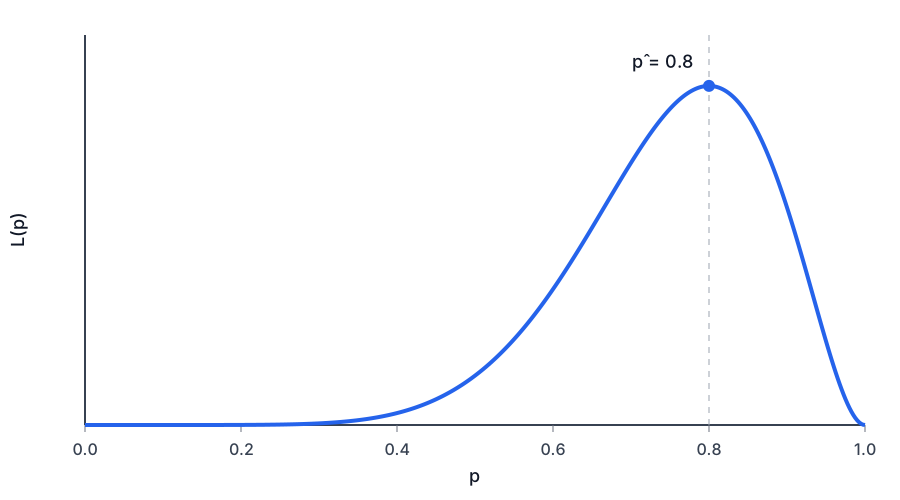
The small vertical values are probabilities of a particular ordered sequence. MLE compares candidates for the same data; it does not require the winning likelihood to be close to one.
Setting p to 1 would make the two tails impossible, so its likelihood is zero. Seeing more heads does not mean assigning heads probability one.
If we recorded only the number of heads, rather than the ordered sequence, a binomial coefficient would also appear. That factor is independent of p and leaves the maximizing parameter unchanged.
Maximum likelihood is an estimation principle, not a consequence forced on us by Softmax. It also does not guarantee a well-generalizing model. Here we are constructing a training objective, not proving that its optimum is the best possible predictor outside the sample.
Why the logarithm, and why the minus sign?
For positive numbers,
\[\log(ab)=\log a+\log b.\]Since the natural logarithm is strictly increasing, taking it preserves the maximizing parameters wherever likelihood is positive:
\[\operatorname*{arg\,max}_\theta L(\theta;D)=\operatorname*{arg\,max}_\theta\log L(\theta;D).\]Zero likelihood can be assigned log-likelihood minus infinity by a limiting convention. For the coin, at interior p values,
\[\log L(p;D)=8\log p+2\log(1-p).\]Differentiating and setting the derivative to zero gives
\[\frac{8}{p}-\frac{2}{1-p}=0.\]Hence
\[\widehat p=\frac8{10}=0.8.\]The second derivative is negative throughout the interval, and the endpoint likelihoods are zero:
\[\frac{d^2}{dp^2}\log L(p;D)=-\frac8{p^2}-\frac2{(1-p)^2}<0.\]So this is the unique maximum. In this Bernoulli example, MLE recovers the empirical frequency.
The logarithm also helps computation: products of many small probabilities can underflow, whereas we can accumulate their logs without first forming the product. Taking a log after the product has already rounded to zero cannot recover the lost information.
Finally, a maximization can be rewritten as a minimization by changing the sign:
\[\mathcal L_{\mathrm{NLL}}(\theta;D)=-\log L(\theta;D).\]This is negative log-likelihood. The log turns products into sums; the minus sign turns maximization into minimization.
For one observed outcome assigned probability p, the contribution is
\[\ell(p)=-\log p,\qquad 0<p\leq1.\]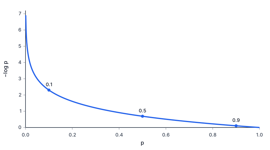
The curve is drawn from p = 0.001 to p = 1. At p = 0 the loss has no finite value. The marked probabilities 0.1, 0.5, and 0.9 give losses approximately 2.303, 0.693, and 0.105.
A high assigned probability gives a small loss. A tiny assigned probability gives a large loss. The curve describes the training penalty, not a separate guarantee that the prediction was calibrated.
The language-model objective, and its implementation
Take N training sequences of the fixed length T used above, retaining repeated sequences as repeated observations:
\[D=\left(x_{1:T}^{(1)},\ldots,x_{1:T}^{(N)}\right).\]Modeling them as independent draws from the same sequence model gives
\[L(\theta;D)=\prod_{n=1}^{N}P_\theta\left(x_{1:T}^{(n)}\right).\]The chain rule then gives
\[L(\theta;D)=\prod_{n=1}^{N}\prod_{t=1}^{T}P_\theta\left(x_t^{(n)}\mid x_{<t}^{(n)}\right).\]The outer product uses an independence assumption across examples. The inner product uses the chain rule within a sequence. They are not the same assumption written twice.
Taking the negative log produces
\[\boxed{\mathcal L_{\mathrm{NLL}}(\theta;D)=-\sum_{n=1}^{N}\sum_{t=1}^{T}\log P_\theta\left(x_t^{(n)}\mid x_{<t}^{(n)}\right)}\]Each position supplies an observed prefix and the token that followed it. The model predicts a full distribution; the loss selects the probability assigned to that observed token. Observing cats once does not imply that dogs was impossible.
Under this model and loss, next-token training is sequence maximum-likelihood training expressed as a sum of local terms. Dividing by the fixed number of predicted tokens rescales the objective without changing its minimizers. We have not yet derived the optimizer or promised that it will find a global optimum.
The implementation also matters. Softmax’s shift invariance lets us subtract the largest logit before exponentiating. For finite float32 or float64 inputs with a nonempty last axis, this teaching implementation also handles batches:
import torch


def softmax_stable(x: torch.Tensor) -> torch.Tensor:
    """Normalize finite float32/float64 logits along a nonempty last axis."""
    max_x = x.max(dim=-1, keepdim=True).values
    shifted_x = x - max_x

    exp_x = torch.exp(shifted_x)
    row_sums = exp_x.sum(dim=-1, keepdim=True)

    return exp_x / row_sums
The tensor returned by .values contains the maxima rather than their indices. Keeping that dimension lets subtraction broadcast along the candidate axis. In exact arithmetic this computes the same Softmax; in floating point it avoids large positive exponential arguments. Extremely small weights may still underflow.
When the next operation is a logarithm, computing log(softmax(x)) separately can lose information through those tiny probabilities. PyTorch’s log_softmax computes log-probabilities directly using a more numerically stable formulation.3 Mathematical equivalence alone does not make two floating-point implementations equally reliable.
The companion llm-from-first-principles project is where I work through such implementation details. Here, the distinction worth keeping is simpler: parameterization makes a distribution available; the learning objective tells us how observations should shape it.
One expression now deserves another look:
\[-\log p.\]So far it emerged from likelihood and a convenient transformation. Why is it also called surprisal, or self-information? And what changes when we average it over a distribution rather than evaluate one observation?
That is where the next article begins.
-
Yoshua Bengio, Réjean Ducharme, Pascal Vincent, and Christian Jauvin. A Neural Probabilistic Language Model. Journal of Machine Learning Research, 3:1137–1155, 2003. The paper discusses n-gram sparsity and learning distributed representations jointly with a probability model. ↩
-
Tomas Mikolov, Ilya Sutskever, Kai Chen, Greg Corrado, and Jeffrey Dean. Distributed Representations of Words and Phrases and their Compositionality, 2013. See Section 2 for input/output word vectors and the alternative training objectives. ↩
-
PyTorch documentation: torch.nn.functional.log_softmax. The numerical caveat concerns separately evaluating Softmax and the logarithm. ↩