How Does a Token Read Its Context?

English · 中文 · Français

First Principles of LLMs & RL · Article 06 · Previous article

Writing note: The ideas and initial material are mine. ChatGPT assisted with drafting, editing, translation, numerical checks, and the original figures and animation sources.

From a Reading Request to Self-Attention, Queries, Keys, and Values

In the previous article, Felix left a blue notebook in the meeting room. Someone trying to find it cared about the location; someone trying to identify it cared about the color. From that distinction, we developed a reading mechanism: retain a collection of representations, score them using the current state, and combine their information with those weights.

In that encoder–decoder model, the request came from the decoder state. But positions within a sentence may need context too. A pronoun needs to be related to a previously mentioned person; a verb’s representation may need information about its subject.

This time, we will let those positions make the requests. Before giving them the names Query, Key, and Value, though, it helps to take one read apart.

1. Finding information and retrieving it are different jobs

Consider the same sentence:

Felix left the blue notebook in the meeting room yesterday.

Imagine that we manually organize its information into searchable cards. One card has the matching labels “notebook, location” and the content “meeting room.” Another has the labels “notebook, color” and the content “blue.”

To answer “Where is the notebook?”, we first determine which card matches the request, then retrieve what that card provides.

What are we looking for?	What clues help match the record?	What is retrieved?
Where is the notebook?	notebook, location	meeting room
What color is the notebook?	notebook, color	blue

“This is location information” helps us find a record, but does not yet tell us which location. The same kind of matching clue could accompany another card whose content is “office.”

The features used to find information need not be the content transmitted once it is found.

Now name the three roles.

The Query is the current reading request. Here, it expresses that we are looking for the notebook’s location.

The Key is the representation through which candidate content participates in matching. Here, “notebook, location” provides clues to compare with the request.

The Value is what that candidate supplies when read. Here, it tells us that the particular location is the meeting room.

This table is a hand-organized retrieval analogy. A real model does not first turn the sentence into cards with human-readable labels. In a Transformer, Queries, Keys, and Values are vectors; learnable computations establish their matching relationships and transmitted content.¹

What the analogy preserves is a distinction of function, not the labels themselves. A Key and a Value may contain overlapping information. They are not necessarily a “short version” and a “complete version” of some content. Separating the roles simply allows the model to learn suitable representations for matching and transmission separately.

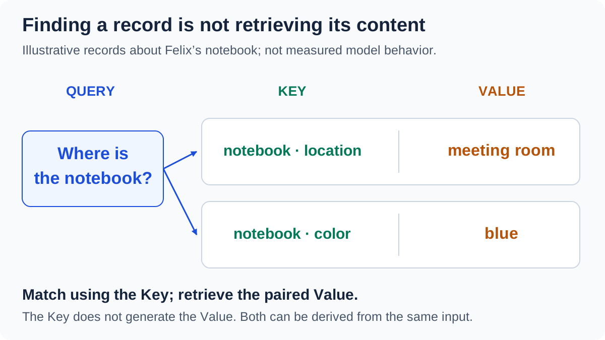
The cards illustrate functions, not manually assigned semantic labels inside a model. The request-first visual explanation is informed by 3Blue1Brown’s attention video; all figures, numerical examples, and animation code here are original.²

2. When the request comes from inside the sentence

So far, an external reader has asked the question. Extend the sentence slightly:

Felix left the blue notebook in the meeting room because he was in a hurry.

For a human reader, Felix provides a clue for interpreting he. This suggests a model-design requirement: the position processing he should have a way to read earlier information about a person.

Using the same roles, we can describe the intended behavior roughly: the position containing he issues a request for relevant person information; earlier positions supply clues for comparison; the read brings back some vector information about candidate people for subsequent computation.

This does not assume that the model literally produces the sentence “Find the person this pronoun refers to.” Nor does it claim that one attention operation completes coreference resolution. It is an example of an information need, not an observation from a trained model. The “request” must ultimately be computed from the representation already available at the current position.

Each position can therefore have two roles. As a reader, it requests information from other positions. As an information source, it offers a Key and a Value to other readers.

When requests and retrieved content come from the same set of sequence representations, this organization is called Self-Attention. Self refers to their common source, not to a rule that a position may read only itself. When the request comes from a decoder and the content comes from an encoder, the read crosses sequences and is generally called Cross-Attention.¹

This is separate from the choice of matching rule. We can ask where requests originate, then independently choose additive or dot-product scoring. Self-Attention does not logically force one particular scoring equation.

Recall Article 04’s I like and They like. If like has the same token ID and position, an independent embedding lookup plus the same positional vector still produces the same initial representation.

That does not force the next result to be identical. The same initial request can retrieve different content when it encounters different Keys and Values. A model does not have to understand the entire context before it can begin reading it.

3. Turning the roles into learnable computations

Start with one position.

Let xᵢ be the vector at position i at the entrance to the current layer, with representation width d_model. Following the previous article, individual position vectors are columns:

\[x_i\in\mathbb R^{d_{\mathrm{model}}}.\]

At the first layer, this can combine a token embedding and positional information. Deeper in the model, it is the result of preceding computations. Here xᵢ is a vector, not a discrete token ID.

A simple learnable way to give the same input three roles is to use three linear projections. Denote their parameters by W_Q, W_K, and W_V:

\[q_i=W_Q^\top x_i, \qquad k_i=W_K^\top x_i, \qquad v_i=W_V^\top x_i.\]

A linear projection recombines input coordinates. It need not know in advance which coordinate means “person” or “place.” Training determines whether the projections form useful matches and content representations. Here we study one set of projections and its basic read, omitting biases, dropout, and the subsequent output projection.¹

Let d_k be the dimension of Queries and Keys, and d_v the dimension of Values. The parameter shapes are:

\[W_Q,W_K\in\mathbb R^{d_{\mathrm{model}}\times d_k}, \qquad W_V\in\mathbb R^{d_{\mathrm{model}}\times d_v}.\]

Queries and Keys must have the same dimension for the direct dot product below. Values do not participate in that dot product, so their dimension can be chosen separately.

One distinction is easy to miss: each position has its own Query vector, but not its own independent set of Query parameters. All positions in this layer use the same W_Q. The Key and Value projections similarly share their respective parameters. Different inputs can produce different vectors.

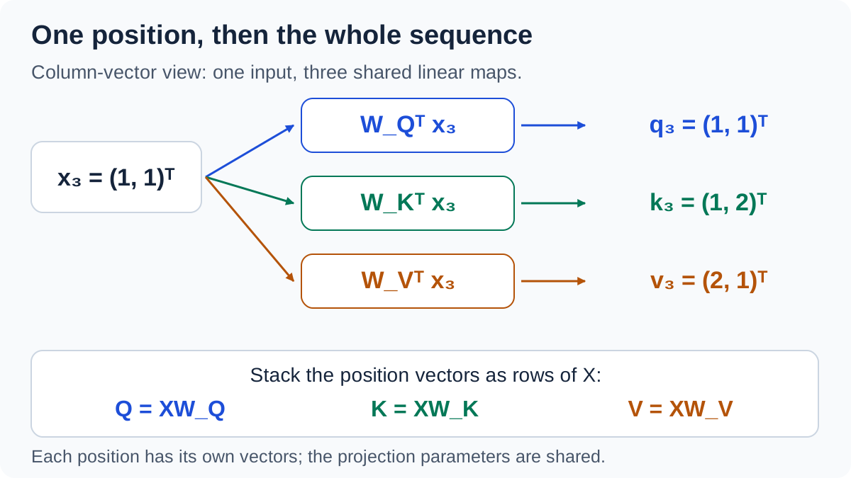
Individual vectors are columns; the full sequence stacks their transposes as rows. The constructed input x₃ illustrates the three roles without assigning word meanings to its coordinates.

How does a request match a candidate?

For the request qᵢ at position i and the candidate clue kⱼ at position j, consider the dot product:

\[q_i^\top k_j = \sum_{r=1}^{d_k}q_{ir}k_{jr}.\]

If we temporarily imagine coordinates as comparable features, this operation multiplies the request’s orientation on each coordinate by the candidate’s corresponding value, then adds the contributions.

That explains the operation, not the interpretation of a trained representation. It does not guarantee that individual coordinates have nameable linguistic meanings. The dot product also depends on vector magnitudes; it is not automatically semantic similarity.

Substituting the projections makes the trainable part visible:

\[q_i^\top k_j = x_i^\top W_QW_K^\top x_j.\]

The inputs are not simply compared in a fixed, inherently correct semantic space. The learned matrices determine how input directions participate in matching.

In the language example, the relationship between he and Felix is not merely that the words are similar. One position needs relevant person information; another may supply it. The desired relationship is useful compatibility for this read, not simply resemblance to the current word.

We could also omit the independent projections and directly take inner products between input vectors. But their raw scores would satisfy:

\[x_i^\top x_j=x_j^\top x_i.\]

Independent Query and Key projections do not require this symmetry. They allow the raw matching relation for “position i reads position j” to differ from the reverse relation. This concerns raw scores: even symmetric scores can produce asymmetric attention weights after row-wise normalization, because different rows may have different denominators.

Separating Values answers another question. Even after deciding which position to read, the content supplied downstream need not use the same coordinates that produced the match.

4. From matching scores to a read

The dot product supplies a score, not yet a final mixing coefficient. First consider its scale; then consider how the scores should combine content.

Why adjust the scale as the dimension increases?

The previous article already used Softmax. It is sensitive to relative score gaps: sufficiently large gaps can concentrate weight on a few positions.

The number of products in a dot product grows with the Query/Key dimension. To isolate that effect, suppose, for this idealized analysis, that all components of q and k are mutually independent, with zero means and unit variances.

For the product at one coordinate:

\[\mathbb E[q_rk_r]=0, \qquad \mathbb E[q_r^2k_r^2] = \mathbb E[q_r^2]\mathbb E[k_r^2] =1.\]

Therefore:

\[\operatorname{Var}(q_rk_r)=1.\]

Products at different coordinates are also independent under these assumptions, so their variances add:

\[\operatorname{Var}(q^\top k)=d_k, \qquad \operatorname{Std}(q^\top k)=\sqrt{d_k}.\]

Notice what adds with dimension: variance. Standard deviation is its square root. This is why the scaling involves a square root rather than the dimension itself.

Dividing by that standard-deviation scale gives unit variance under the stated assumptions:

\[\operatorname{Var}\!\left(\frac{q^\top k}{\sqrt{d_k}}\right)=1.\]

Define the score used for reading as:

\[e_{ij}=\frac{q_i^\top k_j}{\sqrt{d_k}}.\]

This is the original Transformer’s motivation for scaled dot-product attention: prevent increased dimension alone from pushing Softmax toward regions with very small gradients. Real Queries and Keys arise from learned representations and may even come from the same position. They need not meet the independence assumptions, and the scaling does not guarantee unit-variance scores throughout training.¹

Could we multiply the scores directly by the Values?

Yes. We would simply need to accept the properties of that choice.

Take a scalar example unrelated to language. Two candidates have scores 2 and 1; their Values are 10 and 20. Treating the scores directly as coefficients gives:

\[o_{\mathrm{raw}}=2\times10+1\times20=40.\]

Add 100 to both scores. Their gap remains 1, but the result becomes:

\[o_{\mathrm{raw}}'=102\times10+101\times20=3040.\]

There is no mathematical contradiction. Raw-score mixing uses both the absolute baseline and the relative gaps of the scores.

If a read should depend only on relative scores, we need another map from scores to coefficients. Softmax is one choice. Denote the weight assigned by position i to candidate j by aᵢⱼ:

\[a_{ij} = \frac{\exp(e_{ij})}{\sum_{m=1}^{n}\exp(e_{im})}.\]

Here n is the number of candidate positions. For now, assume all are visible, their scores are finite, and at least one candidate exists. Then:

\[a_{ij}>0, \qquad \sum_{j=1}^{n}a_{ij}=1.\]

Softmax is insensitive to a common offset, so our two score vectors yield the same weights:

\[\operatorname{softmax}([2,1]) = \operatorname{softmax}([102,101]) \approx[0.731059,\;0.268941].\]

The retrieved content becomes:

\[o \approx 0.731059\times10+0.268941\times20 \approx12.689414.\]

This chooses a normalized read rather than an arbitrary linear mixture. For fixed Values, nonnegative coefficients summing to one make the result a convex combination. For vector Values, it lies in their convex hull. It cannot grow arbitrarily merely because the coefficients’ sum grows.

This does not prove that every attention mechanism must use Softmax. We can choose a different score-to-weight mapping and examine whether it allows negative coefficients, normalizes them, and controls output scale. A legal matrix operation and a desired reading behavior are different considerations.

Article 02 offered another perspective: allocating probability while trading off high scores against entropy yields a Softmax form. Replacing the fixed action values there with matching scores here gives the same mathematical structure. That interprets the allocation rule for fixed scores; it does not mean that attention separately runs an RL training procedure.

Why does the request not disappear during normalization?

Article 05 contained a counterexample. Removing tanh from its additive scorer left only a linear sum of a request term and a candidate term. The request’s contribution became a shared offset across all candidates, which Softmax removed.

Here the interaction is multiplicative. For two visible candidates j and m, the Softmax ratio gives directly:

\[\begin{aligned} \log\frac{a_{ij}}{a_{im}} &=e_{ij}-e_{im}\\ &=\frac{q_i^\top(k_j-k_m)}{\sqrt{d_k}}. \end{aligned}\]

Changing the Query can change the candidates’ relative scores and, therefore, their relative reading weights. It is no longer restricted to adding the same offset everywhere.

This is one way to make the request and candidate jointly determine a score, not the only possible replacement for additive scoring. If the two Keys are identical, no Query can distinguish them using this rule. If a Query change is orthogonal to their difference, their relative weight will not change either.

Finally, retrieve the content using these weights:

\[o_i=\sum_{j=1}^{n}a_{ij}v_j.\]

In the card analogy, the Key helps decide whether the record matches; the Value determines what that record contributes. Softmax does not alter that division of labor. It allows a continuous mixture of candidates instead of first making a hard choice of one card.

5. Computing all positions together

So far, we have followed one reader. A full sequence repeats the same kind of read.

Let the current sequence contain n token positions. Transpose the input column vectors and stack them as rows:

\[X= \begin{bmatrix} x_1^\top\\ x_2^\top\\ \vdots\\ x_n^\top \end{bmatrix} \in\mathbb R^{n\times d_{\mathrm{model}}}.\]

Here n is the current sequence length, not the tokenizer’s vocabulary size.

Apply the same projections to every row:

\[Q=XW_Q, \qquad K=XW_K, \qquad V=XW_V.\]

Each row of Q, K, and V holds the transpose of one Query, Key, or Value. Their shapes are:

\[Q,K\in\mathbb R^{n\times d_k}, \qquad V\in\mathbb R^{n\times d_v}.\]

“Per token” and “for the whole sequence” are not competing explanations. Mathematically, each position independently applies the shared projections; computationally, those operations can be batched into matrix multiplications. These projections do not themselves mix positions within this layer. Comparing all Queries with all Keys produces the position-to-position interaction of this read.

Collect the scores, normalize each row, and retrieve the Values:

\[\boxed{ O= \operatorname{softmax}_{\mathrm{row}}\!\left( \frac{QK^\top}{\sqrt{d_k}} \right)V }\]

QKᵀ has shape n × n. Row i contains reader i’s scores for all candidates; column j records how all readers score candidate j. O has shape n × d_v, with one retrieved vector per row.³

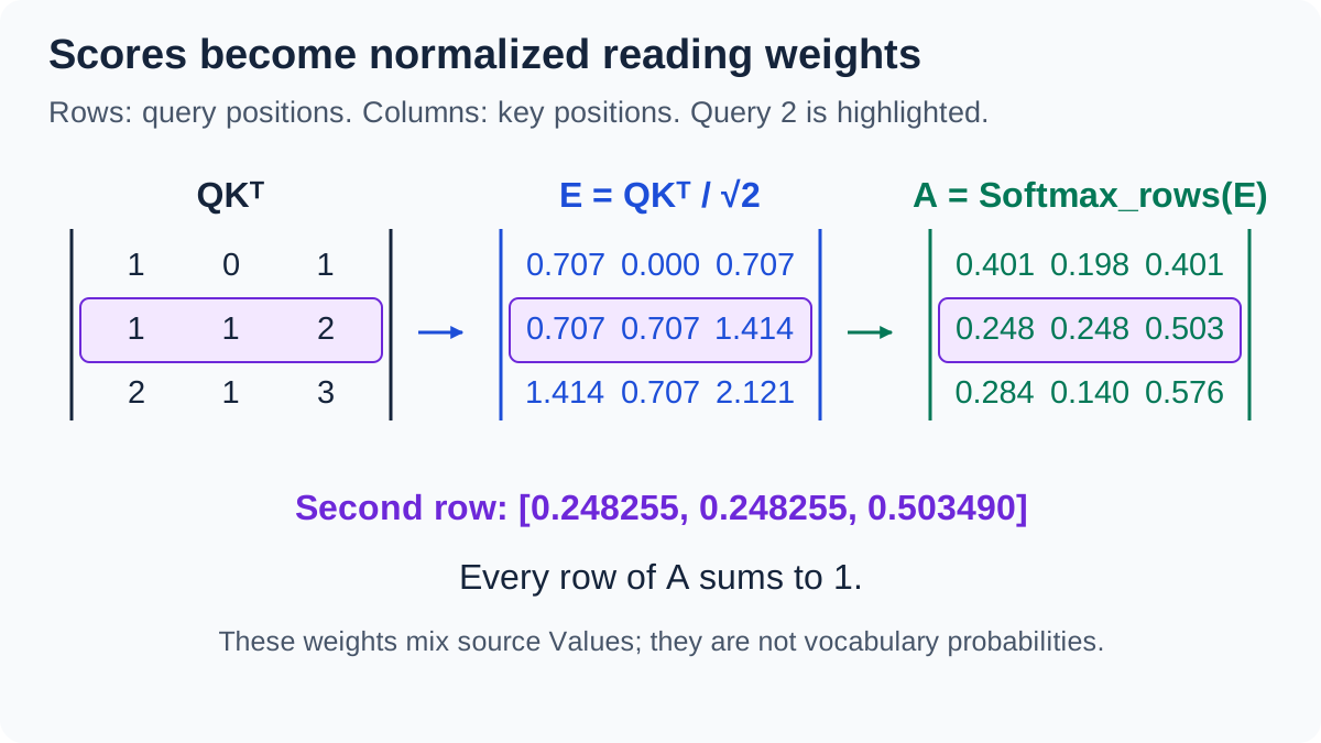
This previews the complete example below. All three rows are divided by √2 before separate normalization; purple highlights Query 2.

Recomputing a three-position example

Now calculate a constructed example. The positions are numbered; we will not present them as actual embeddings of Felix, notebook, or meeting room. Every input and projection matrix is specified by hand.

Use three positions and two-dimensional inputs, Queries, Keys, and Values:

\[n=3, \qquad d_{\mathrm{model}}=d_k=d_v=2.\]

The inputs and parameters are:

\[X= \begin{bmatrix} 1&0\\ 0&1\\ 1&1 \end{bmatrix}, \qquad W_Q= \begin{bmatrix} 1&0\\ 0&1 \end{bmatrix},\] \[W_K= \begin{bmatrix} 1&1\\ 0&1 \end{bmatrix}, \qquad W_V= \begin{bmatrix} 2&0\\ 0&1 \end{bmatrix}.\]

Therefore:

\[Q= \begin{bmatrix} 1&0\\ 0&1\\ 1&1 \end{bmatrix}, \qquad K= \begin{bmatrix} 1&1\\ 0&1\\ 1&2 \end{bmatrix}, \qquad V= \begin{bmatrix} 2&0\\ 0&1\\ 2&1 \end{bmatrix}.\]

First calculate all dot products:

\[QK^\top= \begin{bmatrix} 1&0&1\\ 1&1&2\\ 2&1&3 \end{bmatrix}.\]

Follow only position 2. Its scaled scores for the three candidates are:

\[e_2= \frac{1}{\sqrt2}[1,1,2] \approx[0.707107,\;0.707107,\;1.414214].\]

Softmax gives:

\[a_2\approx[0.248255,\;0.248255,\;0.503490].\]

Combine the three Values with these coefficients:

\[\begin{aligned} o_2 &\approx 0.248255\begin{bmatrix}2\\0\end{bmatrix} + 0.248255\begin{bmatrix}0\\1\end{bmatrix} + 0.503490\begin{bmatrix}2\\1\end{bmatrix}\\ &\approx \begin{bmatrix} 1.503490\\ 0.751745 \end{bmatrix}. \end{aligned}\]

Key coordinates produced the coefficients; Value coordinates are what get added. Holding Q/K fixed while changing Values leaves the weights unchanged but can change the retrieved vector.

Even a 70% mixing weight does not mean a position has a 70% probability of being the “correct explanation.” The weights describe this read’s combination coefficients; they do not independently calibrate semantic correctness.

Nor are they next-token probabilities. Their candidates are input positions, not vocabulary entries. Here o₂ is a two-dimensional vector. Subsequent computation must still turn the model’s representation into a prediction over the vocabulary.

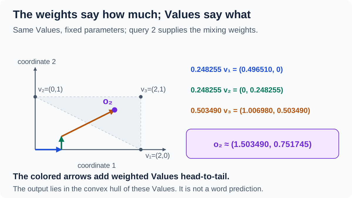
The colored arrows show vector addition within one forward computation, not a training trajectory. Calculations use full precision; displayed numbers are rounded.

6. Computing together does not permit reading the future

The preceding example allowed every position to read every other position. That illustrates reading a complete input, but not the visibility rule required for autoregressive generation.

To avoid index confusion, let t₁ through tₙ denote discrete input tokens, while xᵢ still denotes the corresponding vector. Adopt this prediction convention: position i has received token tᵢ, and its representation helps predict the next token, tᵢ₊₁. The target conditional distribution is:

\[p_\theta(t_{i+1}\mid t_{1:i}).\]

Position i can therefore read itself and earlier positions, but not the next position, which would already contain the answer.

During training, the full text is present in the dataset, but the model must still respect that constraint. The original Transformer combines an offset between input and target tokens with masking of forbidden attention connections.¹

Under our indexing convention, define a causal mask:

\[M_{ij}= \begin{cases} 0,&j\le i,\\ -\infty,&j>i. \end{cases}\]

Then compute:

\[A= \operatorname{softmax}_{\mathrm{row}}\!\left( \frac{QK^\top}{\sqrt{d_k}}+M \right).\]

The exponential corresponding to negative infinity is zero, so normalization considers only visible candidates. Every row must retain at least one visible position. Allowing self-reading satisfies that condition here.

Return to row 2 of our numerical example. Position 3 is no longer visible, so the scores become:

\[\left[ \frac1{\sqrt2}, \frac1{\sqrt2}, -\infty \right].\]

The weights and output become:

\[a_2^{\mathrm{causal}}=[0.5,\;0.5,\;0], \qquad o_2^{\mathrm{causal}}= \begin{bmatrix} 1\\ 0.5 \end{bmatrix}.\]

Previously, the first two weights were about 0.248255 each; now each is 0.5. Once the future is hidden, the remaining positions share all the weight.

This is why merely zeroing future weights after Softmax does not produce the same normalized read. Zeroing and then renormalizing the retained weights is equivalent in exact arithmetic. Here we use the mask-before-Softmax formulation.³

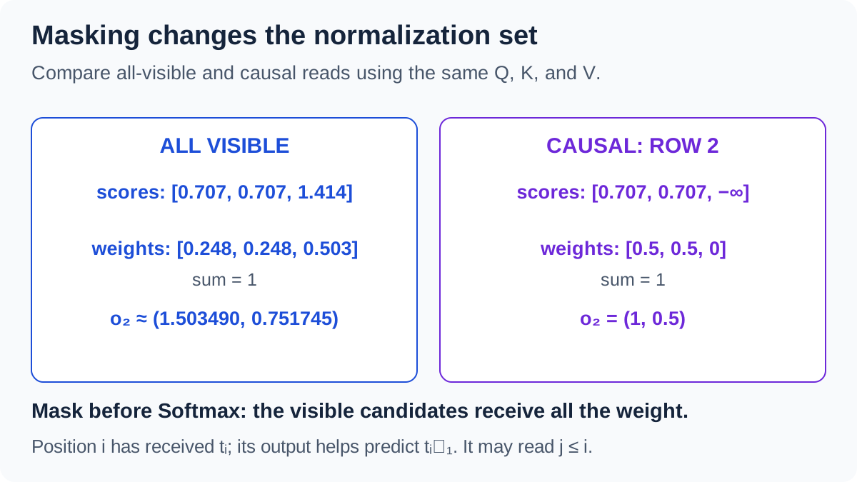
Only the visibility rule changes between the full and causal reads. Position i has received its current token and helps predict the next, so reading itself is allowed.

Which columns a row may read is separate from whether multiple rows can be computed simultaneously. Once this layer’s inputs are ready, positions can compute their reads in parallel while the mask restricts each row’s information sources. Earlier layers in a standard causal model must respect the same kind of visibility constraint. Adding a mask only at the last layer cannot remove future information leaked earlier.

A matrix row number does not, by itself, supply a position representation either. With only the unmasked, position-free content-matching operations above, permuting input rows correspondingly permutes output rows. That permutation equivariance follows directly from the operations; it does not mean the output knows each token’s original position number.

This returns to Article 04: a position mechanism supplies information the computation can use. A causal mask separately restricts which connections can carry information; it is not the same thing as a vector-valued position encoding.

7. Why would these projections learn anything useful?

So far, we have specified a computable structure. Random parameters do not guarantee a link between he and Felix.

The learning signal still comes from the prediction loss used throughout the preceding articles. The read affects the later prediction, the scores affect the read, and Queries and Keys affect the scores. We can follow those dependencies backward to the projection parameters.

Write the loss as L, and denote the column-vector gradient arriving at position i’s read by gᵢ:

\[g_i=\nabla_{o_i}\mathcal L.\]

For this read, temporarily hold Values fixed. Differentiating Softmax and the weighted sum gives, for a visible candidate j:

\[\frac{\partial\mathcal L}{\partial e_{ij}} = a_{ij}\,g_i^\top(v_j-o_i).\]

This is the same local relationship as in Article 05. Increasing a candidate’s score pulls the read a little toward its Value. The incoming gradient determines how that change would affect the loss.

Dot-product scoring provides the next steps backward:

\[\nabla_{q_i}e_{ij}=\frac{k_j}{\sqrt{d_k}}, \qquad \nabla_{k_j}e_{ij}=\frac{q_i}{\sqrt{d_k}}.\]

The gradient can then pass through the projections into W_Q and W_K. The Value projection receives gradients through the retrieved content’s effect on the loss.

These are local derivatives of the operations written here. Full training combines contributions from other positions, computational paths, and samples. There is no guarantee that an individual parameter update makes a weight better match a human grammatical interpretation.

Prediction is supervised; reading receives a learning signal through its effect on prediction.

Return to I like and They like. The initial representation of like can be identical, yet different available context can produce a different read. The computation starts with shared projections, performs content-dependent matching, and returns a vector that depends on visible context.

That vector is not yet the complete updated representation. What happens to the information the position already had? Can one set of reading weights serve several different relationships? How does retrieved content enter the next layer?

The next article places this read inside a Transformer block that can preserve an input path, combine several reads, and continue transforming the information.

The examples, figures, and animations are not trained-model results. Reproduce numerical and gradient checks · Static figure generator · Shared numerical inputs.